Combining Professional Forecasters with Copulas (Part 3): A Walk-Forward Horserace

This is the third post in the series. Part 1 introduced the Survey of Professional Forecasters data. Part 2 developed two copula-based ways to combine point forecasts. This post asks how those ideas behave in a walk-forward empirical test.

The empirical results do not identify a single dominant copula method. In this quarterly macro setting, the strongest methods are mostly parsimonious. The nowcast is hard to beat. Error GLS and shrunk Error GLS perform well because they concentrate on the most informative horizon while correcting for redundant and correlated forecast errors. More flexible copula methods are informative diagnostics, but in this sample their additional flexibility does not translate into better out-of-sample forecasts.

From the first two posts to this horserace

Part 2 separated two probability questions.

The outcome-forecast approach models the joint distribution of the realised outcome and the forecasts:

\[(Y, X_1, \ldots, X_D).\]

Its question is:

\[\mathbb{E}[\text{outcome rank} \mid \text{forecast ranks}].\]

The forecast-error approach models the dependence structure of the forecast errors:

\[E_k = X_k - Y.\]

Its question is:

\[\text{which candidate } y \text{ makes } (X_1-y,\ldots,X_D-y) \text{ plausible?}\]

These two questions can lead to similar linear formulas under restrictive Gaussian assumptions, but they are not the same statistical object. The distinction matters once we evaluate rank skill, level accuracy, nonlinear dependence, and different point summaries of a likelihood.

The target is now an official realised value

Parts 1 and 2 used an SPF-aligned proxy target constructed from the available survey panel. For the final horserace I rebuild the panel from the Philadelphia Fed’s official SPF evaluation files. This gives a more precise target definition.

For each variable, the panel contains three realised values:

Target	Meaning
target_initial	first official realised value used for real-time evaluation
target_latest	latest revised official value
target_spf_proxy	earlier proxy target used in Parts 1 and 2

The main experiment uses target_initial. This is closest to the real-time question: what would the forecast have predicted before later data revisions?

I keep target_latest for a revision-sensitivity check. This matters because macro realised values are revised. A forecasting method can look different depending on whether we score it against first releases or later vintages.

The official-target panel covers RGDP, NGDP, PGDP, UNEMP, CPI, INDPROD, and HOUSING. I exclude CPROF from the main horserace because the same aligned official evaluation structure is not available, and the CPROF definition changes over time.

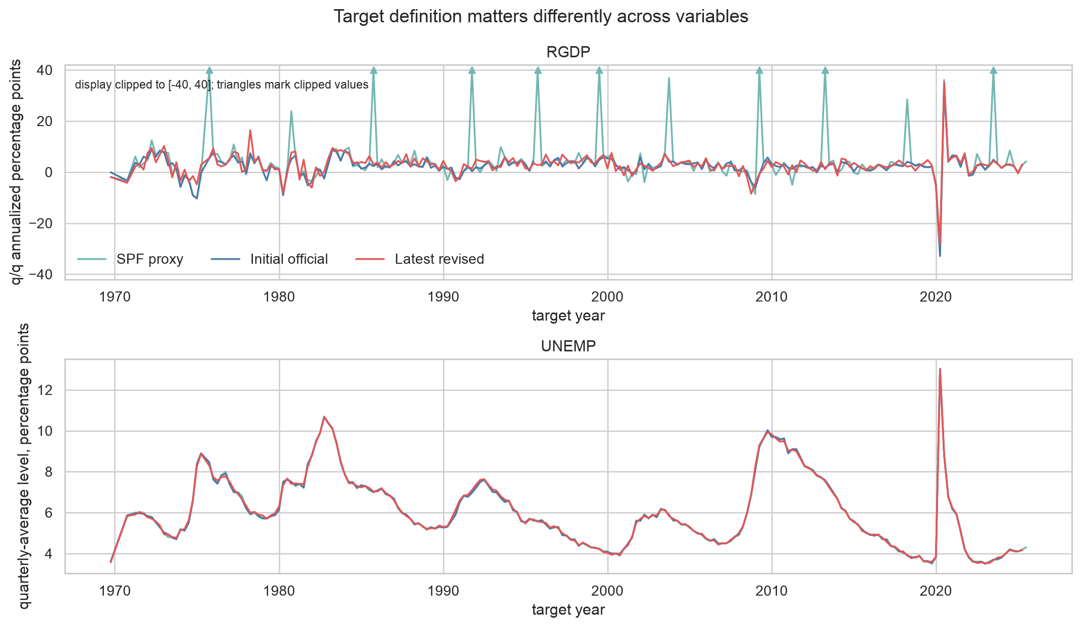
The figure shows why this matters. For unemployment, the different target definitions are almost identical in rank. For growth variables, especially RGDP, the proxy, initial release, and latest revised value can differ materially.

Evaluation design

The main experiment is a walk-forward expanding-window evaluation.

For each target date, a method is trained only on information from earlier target dates. The training window then expands by one date and the procedure repeats. This is closer to the way a forecast-combination method would be used in practice than a single fixed train/test split.

The cross-horizon experiment combines SPF consensus forecasts made at leads 0 through 4 for the same target. Lead 0 is the nowcast. Longer leads are progressively earlier forecasts for the same realised quarter.

The methods are:

Family	Methods
Simple benchmarks	persistence, Lead 0, equal weight, trimmed mean, inverse MSE
Outcome-forecast dependence	OLS on raw ranks, Gaussian outcome copula, shrunk Gaussian outcome copula, truncated outcome vine
Forecast-error dependence	Error GLS, shrunk Error GLS, Gaussian error copula, vine error copula

The rank metric is computed as follows. Actuals and predictions are ranked separately within each macro variable, then those within-variable ranks are stacked and one Spearman correlation is computed. This avoids comparing the level of unemployment directly with the level of GDP growth, while still giving one summary number for the full panel.

The level metric is scaled RMSE. Each error is divided by the standard deviation of the realised target in the training sample for that variable. This makes the level errors roughly comparable across variables with different units. Scaled bias is the average scaled error, so positive values mean the method tends to overpredict.

The main result

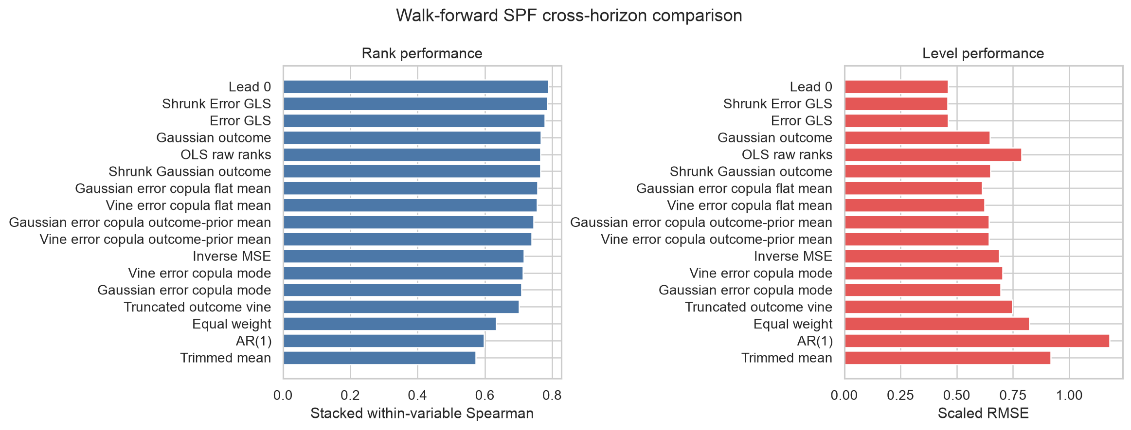
The main table is below. Higher rank correlation is better. Lower scaled RMSE is better.

Method	Stacked rank rho	Scaled RMSE	Scaled bias
Lead 0	0.788	0.461	-0.005
Shrunk Error GLS	0.786	0.459	-0.007
Error GLS	0.778	0.461	-0.004
Gaussian outcome copula	0.766	0.647	0.014
OLS raw ranks	0.766	0.788	0.054
Gaussian error copula, flat mean	0.757	0.612	0.033
Vine error copula, flat mean	0.755	0.623	-0.003
Inverse MSE	0.716	0.689	0.043
Truncated outcome vine	0.702	0.746	-0.087
Equal weight	0.634	0.822	0.061
Persistence	0.598	1.179	0.017
Trimmed mean	0.573	0.919	0.067

The persistence benchmark is the last observed realised value available in the expanding training sample. The strongest benchmark is not a sophisticated model. It is Lead 0, the nowcast. In this cross-horizon setting there is a structural skill hierarchy: the forecast made closest to the target quarter contains much more information than the forecasts made several quarters earlier.

The first three rows are very close. Lead 0 has the highest rank correlation, while shrunk Error GLS has the lowest scaled RMSE by a small margin. The nowcast and the two Error GLS variants are therefore broadly comparable at the top of the table. A paired quarter-block bootstrap gives the same interpretation: the gap between Lead 0 and shrunk Error GLS is small relative to sampling variation. Each row below is computed as the first method minus the second method. For RMSE, negative values favour the first method.

Comparison	Delta rank rho	95% bootstrap interval	Delta scaled RMSE	95% bootstrap interval
Lead 0 minus shrunk Error GLS	0.003	[-0.004, 0.009]	0.003	[-0.023, 0.029]
Lead 0 minus Error GLS	0.009	[-0.005, 0.027]	0.001	[-0.068, 0.058]
Lead 0 minus Gaussian outcome copula	0.021	[0.007, 0.035]	-0.172	[-0.367, -0.036]

The ranking against equal-weight is less ambiguous. Relative to equal-weight, Lead 0, shrunk Error GLS, Error GLS, and the Gaussian outcome copula all have positive bootstrap intervals for rank correlation and negative intervals for scaled RMSE.

The Gaussian outcome copula remains a strong rank predictor, but its level RMSE is worse. This level score combines two separate steps: estimating the conditional rank, then mapping that rank back to a level using the empirical training distribution of realised outcomes. The weaker RMSE can therefore come from the marginal calibration and inverse-rank mapping, even when the dependence model orders outcomes well.

Why Error GLS holds up

Error GLS estimates the covariance matrix of forecast errors,

\[\Sigma_E = \operatorname{Cov}(E_1,\ldots,E_D),\]

and uses its inverse, the precision matrix, to form

\[\hat y = \frac{\mathbf{1}^{\top}\Sigma_E^{-1}x} {\mathbf{1}^{\top}\Sigma_E^{-1}\mathbf{1}}.\]

This formula has a simple interpretation. Forecast directions with high error variance count less. Forecast directions that duplicate the same error information also count less. When several horizons are highly correlated, Error GLS avoids treating them as independent pieces of evidence.

The estimated weights make this visible. Averaged across the walk-forward evaluation, both Error GLS variants put most of the weight on the nowcast. The weights sum to one, but they are not constrained to be positive: Error GLS is correcting correlated forecast errors, not imposing a convex average. The unshrunk estimator uses larger offsetting weights. The shrunk version keeps the same broad pattern, but pulls the secondary weights closer to zero; some average weights can still be negative.

Method	Lead 0	Lead 1	Lead 2	Lead 3	Lead 4
Error GLS, average weight	1.370	-0.352	0.005	-0.136	0.112
Shrunk Error GLS, average weight	1.073	0.007	-0.062	-0.056	0.039

This is also why Error GLS ends up close to Lead 0 in the leaderboard: it mostly learns to trust the nowcast, while using the other horizons as smaller error-correction terms.

This is a relatively low-dimensional object to estimate. A full KDE plus error-copula method is more demanding: it estimates each error marginal distribution, fits a multivariate dependence model, and then solves a one-dimensional prediction problem for each new forecast vector. In this sample, the extra flexibility comes with enough estimation variance to offset much of its potential benefit.

Error-copula point summaries

Part 2 introduced the forecast-error copula through the likelihood of the implied error vector:

\[f_E(X_1-y,\ldots,X_D-y).\]

The most direct point forecast is the likelihood mode:

\[\hat y_{\mathrm{mode}} = \arg\max_y f_E(X_1-y,\ldots,X_D-y).\]

That answers the “most plausible error vector” question. But it is not the only possible point summary. If the evaluation criterion is squared error, a mean of the implied likelihood can be more natural than its mode.

I therefore compare three summaries:

Summary	Definition
Mode	choose the candidate $y$ with maximum error likelihood
Flat-prior mean	average candidate $y$ values using weights proportional to $f_E(X-y\mathbf{1})$
Outcome-prior mean	average candidate $y$ values using weights proportional to $f_E(X-y\mathbf{1}) f_Y(y)$

In this experiment, the flat-prior mean is the best of the flexible error-copula summaries. The outcome-prior mean does not clearly help, probably because it adds another estimated object, the marginal density of $Y$. The mode is conceptually clean, but it is not automatically the best summary for RMSE.

The comparison is similar for the Gaussian error copula and the vine error copula:

Error-copula method	Summary	Stacked rank rho	Scaled RMSE	Scaled bias
Gaussian	Mode	0.709	0.694	0.001
Gaussian	Flat-prior mean	0.757	0.612	0.033
Gaussian	Outcome-prior mean	0.745	0.643	0.065
Vine	Mode	0.714	0.703	-0.042
Vine	Flat-prior mean	0.755	0.623	-0.003
Vine	Outcome-prior mean	0.740	0.644	0.040

The error-copula likelihood ranks candidate outcomes by the plausibility of their implied error vectors. Turning that likelihood into a point forecast requires an additional choice: mode, mean, or another summary matched to the evaluation loss.

By-variable rank correlations

The table below reports Spearman rank correlations computed separately for each macro variable.

Variable	Lead 0	Shrunk Error GLS	Error GLS	Gaussian outcome copula	Gaussian error copula, flat mean	Equal weight
CPI	0.809	0.803	0.793	0.778	0.794	0.642
HOUSING	0.967	0.969	0.973	0.963	0.964	0.894
INDPROD	0.777	0.782	0.774	0.762	0.691	0.485
NGDP	0.693	0.682	0.650	0.616	0.674	0.493
PGDP	0.709	0.710	0.711	0.702	0.715	0.619
RGDP	0.571	0.561	0.554	0.550	0.511	0.336
UNEMP	0.997	0.995	0.994	0.992	0.961	0.964

The result is not driven by a single variable. The near-horizon forecast is strong almost everywhere. The two Error GLS variants are especially competitive for HOUSING, INDPROD, PGDP, and UNEMP, with shrunk Error GLS often close to the best method. The Gaussian outcome copula remains competitive as a rank predictor, but it is generally a little weaker than the nowcast/Error GLS group here, and its rank-to-level conversion performs less well for level accuracy.

This table is mainly a diagnostic for whether the pooled result is driven by one macro series. It is not meant to rank methods precisely within each variable, where several top correlations are very close.

RGDP remains difficult. Equal weighting performs poorly because it averages a relatively informative nowcast with much weaker longer-horizon forecasts. This is exactly the setting where dependence correction helps: the combination method should not treat all horizons as equally informative.

Initial releases versus latest revisions

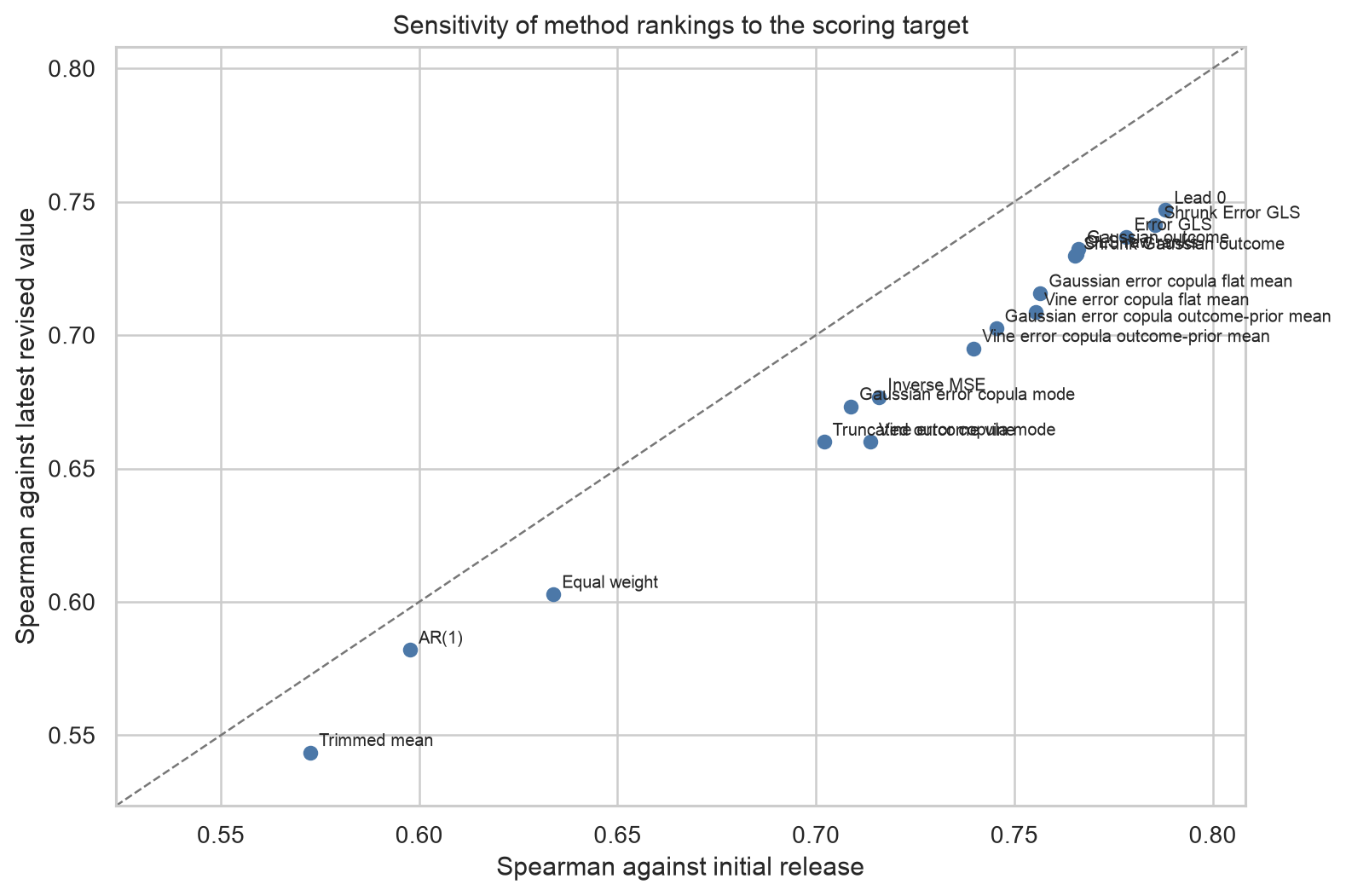
The same predictions can be scored against initial releases or latest revised values. I use the initial release as the main target because it is the first official realised value available after the target period.

I also report the same scores against the latest revised value. This is a useful check because later vintages can reflect additional source data, benchmark revisions, or statistical reprocessing after the initial release.

The broad ranking is similar across the two targets: Lead 0 and Error GLS remain very strong. The level metrics move more than the ranks, especially for the methods closest to the nowcast. This is why I keep the initial-release and latest-revision results side by side.

Method	Rank rho, initial release	Rank rho, latest revised	Scaled RMSE, initial release	Scaled RMSE, latest revised
Lead 0	0.788	0.747	0.461	0.512
Shrunk Error GLS	0.786	0.741	0.459	0.520
Error GLS	0.778	0.737	0.461	0.531
Gaussian outcome copula	0.766	0.732	0.647	0.653
Equal weight	0.634	0.603	0.822	0.821

The deterioration is larger for the top nowcast and Error GLS methods than for equal-weight, because these methods are more tightly tied to the near-term official release. The ordering remains similar, but the target vintage changes the measured size of the advantage.

Rolling performance through time

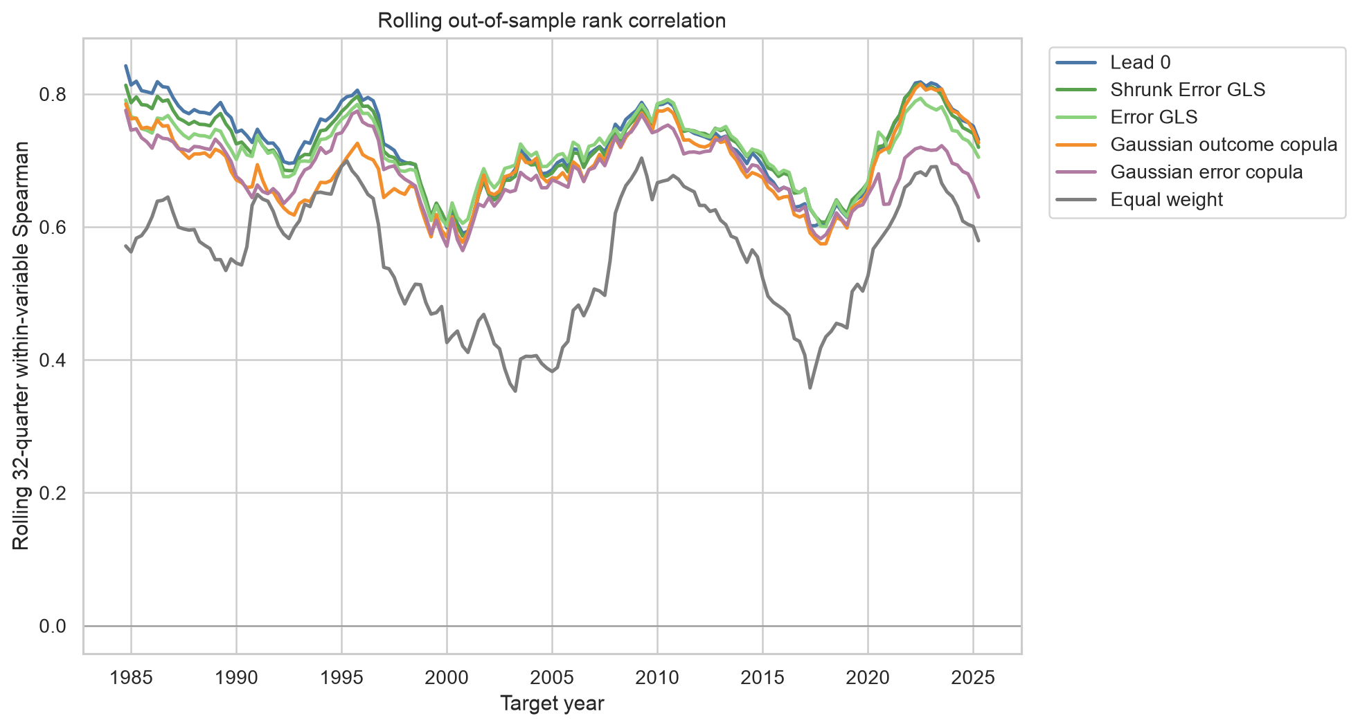
For each target date, the figure computes one within-variable Spearman correlation using the previous 32 quarters of out-of-sample predictions. It is not a pure sample-size experiment. Later fitted forecasts have more training data available, but they are also evaluated in later macroeconomic periods.

Equal weight is a fixed rule, so its line does not move because of re-estimation. It moves because the evaluation window changes. For fitted methods, the rolling lines combine two effects: the training sample expands, and the forecast environment changes.

The main pattern is consistent with the pooled table. Lead 0 and Error GLS remain difficult to separate for much of the sample, while equal weight is usually below them. The gap is not constant through time, which is another reason to treat the single pooled leaderboard as a summary rather than a universal ranking.

Named-forecaster case studies

The cross-horizon experiment has a built-in skill hierarchy: lead 0 is usually more informative than lead 4. The classical forecast-combination puzzle is different. It is often about combining forecasters who make predictions for the same target at the same horizon, with similar information sets and similar skill.

I therefore keep a separate named-forecaster experiment. For CPI, RGDP, and UNEMP, at horizons 1 and 2, I form small panels of individual forecasters and run the same expanding-window evaluation. These variables give three different forecasting problems with enough overlapping individual respondents: inflation, real activity growth, and unemployment. Horizons 1 and 2 keep the comparison at a common forecast horizon while avoiding both the nowcast-dominance issue and the thinner coverage of longer horizons.

The figure uses three-forecaster panels. For each variable-horizon pair, the panels are the three highest-coverage forecaster trios selected before looking at test performance.

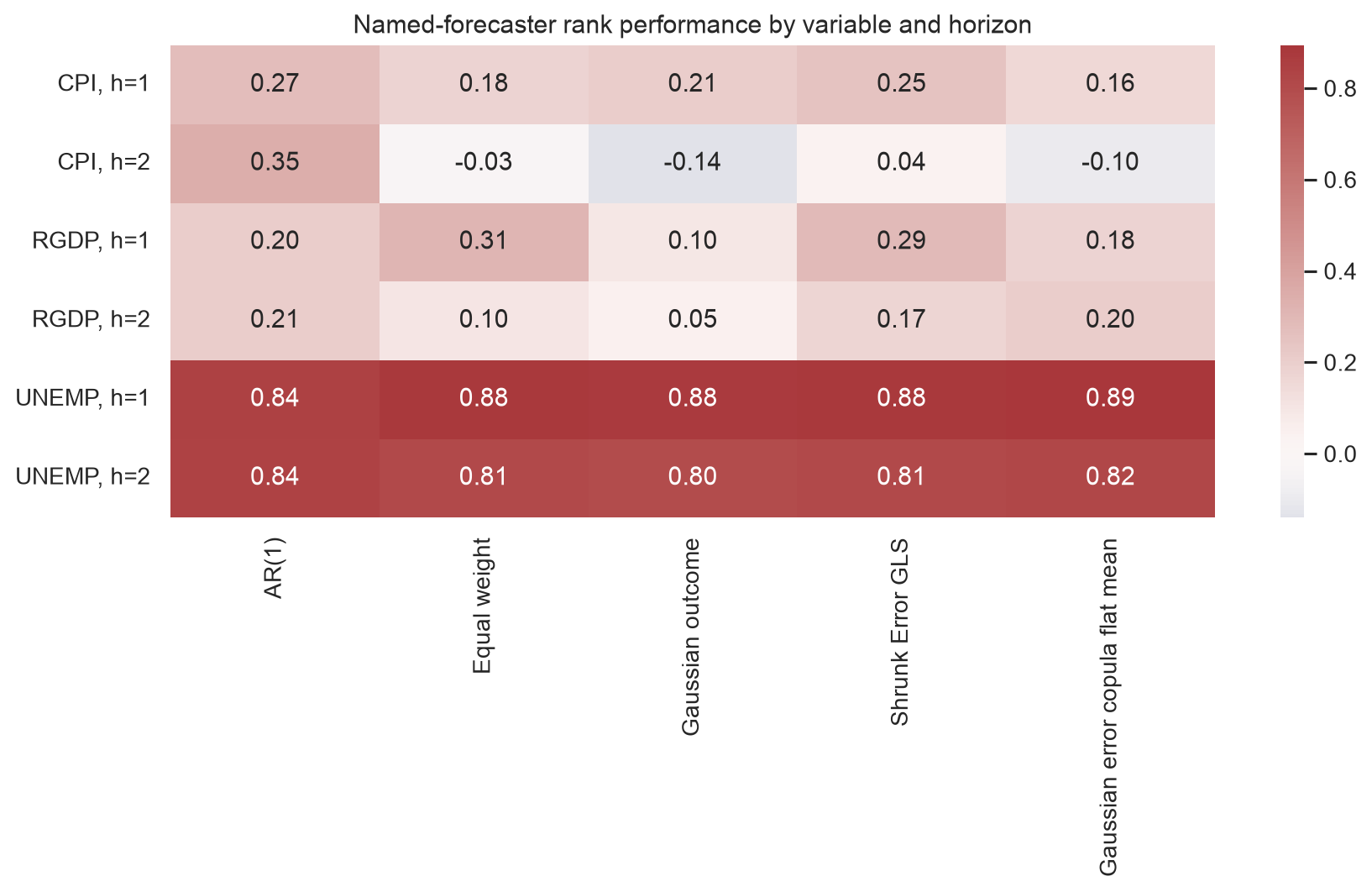
This named-forecaster check is deliberately smaller than the cross-horizon experiment. To get a usable history, I have to reuse many of the same high-coverage forecasters and target dates across panels. The table therefore gives a useful check on how the combination methods behave when the signals are individual forecasters rather than different lead times, but not many independent repetitions of the same experiment. The point is to contrast two empirical settings:

Setting	Main feature
Cross-horizon consensus forecasts	strong structural skill hierarchy across lead times
Named forecasters at the same horizon	closer substitutes with similar information sets

Across these three-forecaster panels, the ranking is much less decisive than in the cross-horizon experiment. The persistence row is the last observed realised value, not a combination of forecasters. The other rows combine the selected forecasters. I round these summaries to two decimals because the panels overlap and the sample is smaller.

Method or benchmark	Named-forecaster rank rho	Scaled RMSE
Persistence	0.51	2.20
Shrunk Error GLS	0.48	1.94
Error GLS	0.47	1.95
Inverse MSE	0.46	1.93
Trimmed mean	0.46	1.93
Equal weight	0.46	1.93
Gaussian error copula, flat mean	0.45	2.03
Gaussian outcome copula	0.39	1.97

I also reran the same construction with four and five forecasters per panel. Larger panels average more individual forecasts, but they leave fewer usable target quarters: every selected forecaster must have reported a forecast for the same variable, horizon, and target quarter. In this SPF sample, that common-overlap constraint makes larger named-forecaster panels quickly lose observations.

Forecasters per panel	Median OOS quarters per panel	Persistence	Inverse MSE	Equal weight	Shrunk Error GLS	Error GLS	Gaussian error copula
3	62	0.51	0.46	0.46	0.48	0.47	0.45
4	46	0.48	0.54	0.54	0.54	0.49	0.47
5	31	0.49	0.49	0.48	0.48	0.42	0.39

The panel-size check does not change the qualitative conclusion. Equal weight, inverse MSE, and shrunk Error GLS remain close to one another, while unshrunk Error GLS and the flexible error-copula do not clearly dominate as the number of forecasters increases. This is closer to the classical forecast-combination puzzle: when forecasters have similar information sets, estimated weights may not improve much on simple regularised averages. Larger panels leave fewer common forecast dates, so I read the table mainly as a robustness check on the named-forecaster exercise.

What I take from the horserace

First, the nowcast is a serious benchmark. In a cross-horizon SPF combination problem, beating Lead 0 is difficult because the nowcast already reflects much of the relevant information.

Second, dependence modeling is still useful. Error GLS and shrunk Error GLS are competitive because they estimate a small, interpretable object: the covariance matrix of forecast errors. That is enough to correct for noisy and redundant horizons.

Third, rank prediction and level prediction are not the same objective. The Gaussian outcome copula is a good rank predictor, but mapping ranks back to levels introduces an additional calibration problem.

Fourth, flexible copulas need enough stable information. The vine and KDE-based error-copula methods can represent richer dependence, but richer models are not automatically better in SPF-sized macro samples.

The empirical exercise preserves the main distinction from Part 2. The results do not select one method that is best in every setting. The copula framework is useful here because it makes two different probability questions explicit:

\[\mathbb{E}[\text{outcome rank} \mid \text{forecast ranks}]\]

is not the same object as

\[\text{the outcome whose implied forecast-error vector is most plausible}.\]

Once those two objects are separated, the empirical results are easier to interpret. In this implementation, the outcome-side methods first estimate ranks and then require a separate rank-to-level calibration step. The error-copula methods search over candidate outcome levels; for each candidate $y$, they compute implied errors $x_k-y$. The copula coordinates are empirical ranks of those implied errors relative to the training errors, while the marginal density terms are estimated with KDE. Error GLS is the parsimonious version of the error-side idea: it uses only an error covariance matrix. In this SPF horserace, the strongest error-side results come from Error GLS and shrunk Error GLS rather than from the KDE plus error-copula methods.