Combining Professional Forecasters with Copulas (Part 2): Two Approaches to Dependence
This is the second post in a three-part series. Part 1 introduced the Survey of Professional Forecasters data. This post builds the modelling framework: two ways to use dependence when combining point forecasts. Part 3 runs the walk-forward empirical horserace on official SPF evaluation targets.
Where this post fits
Part 1 described the raw material: professional forecasters report point forecasts for macro variables such as GDP growth, inflation, unemployment, housing starts, and industrial production at several horizons. For a fixed variable and target quarter, write
\[y_t = \text{realised outcome}, \qquad x_{0,t}, x_{1,t}, \ldots, x_{4,t} = \text{forecasts at leads 0 through 4}.\]In the main SPF experiment, the $x_{k,t}$ are not individual named forecasters. They are the panel consensus forecasts at different lead times: nowcast, one-quarter-ahead, …, four-quarters-ahead. I will use the word “signal” for any predictor being combined: a lead-time consensus, an individual forecaster, or a model output.
There are two natural ways to use copulas here.
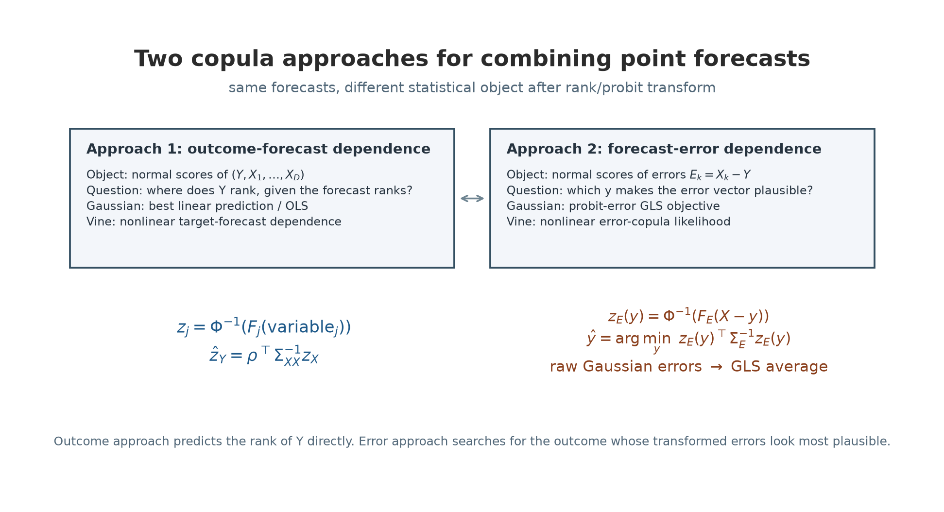
Approach 1: outcome-forecast dependence. Model the joint dependence of
\[(y_t, x_{0,t}, \ldots, x_{4,t})\]after rank transformation. The question is:
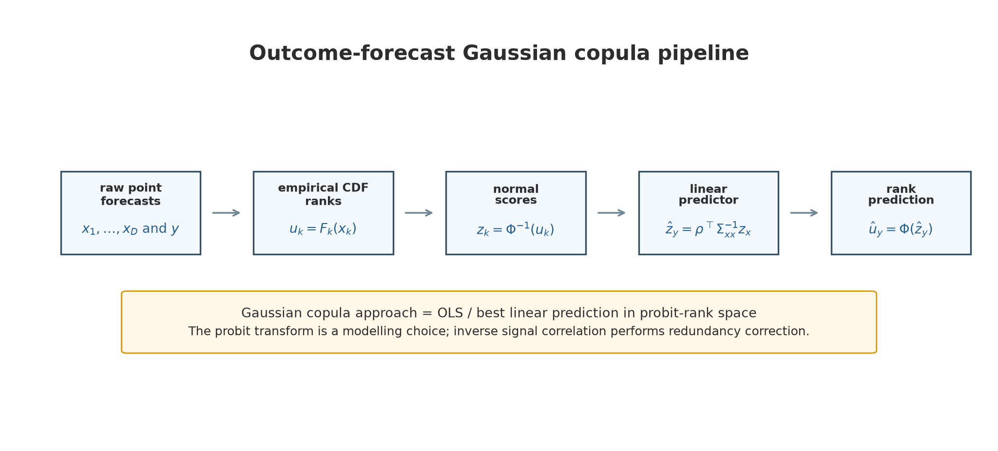
\[\mathbb{E}[y_t \mid x_{0,t}, \ldots, x_{4,t}]?\]In rank space this becomes: given the forecast ranks, what rank should the realised outcome have? The Gaussian copula version reduces to OLS, or best linear prediction, on probit-transformed ranks. A vine copula can replace the Gaussian copula when the target-forecast relationship is nonlinear, asymmetric, or tail-dependent.
Approach 2: forecast-error dependence. Model the joint dependence of forecast errors
\[e_{k,t} = x_{k,t} - y_t.\]The question is different:
\[\hat y_t = \arg\max_y f_E(x_{0,t} - y, \ldots, x_{4,t} - y).\]In words: choose the combined forecast whose implied error vector is most plausible under the learned joint error distribution. This is the direct continuation of my older copula-fusion intuition: learn how predictors err together, then find the value that makes the observed forecasts jointly most likely.
This post is about point forecast ranks and point forecast errors, not full predictive densities. Copulas are often used to combine density forecasts; here they play a narrower role. They model dependence either between outcome and forecasts, or among forecast errors.
Classical forecast combination
Bates and Granger (1969) showed that a weighted average of forecasts can outperform the individual forecasts. For two forecasts with error variances $\sigma_1^2$, $\sigma_2^2$ and error correlation $\rho$, the optimal weight on forecast 1 is
\[w_1^* = \frac{\sigma_2^2 - \rho\sigma_1\sigma_2}{\sigma_1^2 + \sigma_2^2 - 2\rho\sigma_1\sigma_2}.\]The formula already contains the main idea: a good combination needs both individual accuracy and error dependence. If two forecasters make the same mistakes, the second one does not add a full new unit of information.
The practical problem is estimation. Variances and covariances must be learned from finite history. When there are many forecasters, the covariance matrix has many parameters, and the inverse can amplify noise. This is one way the forecast combination puzzle appears: estimated optimal weights often fail to beat the simple average out of sample.
Granger and Ramanathan (1984) proposed regression-based forecast combination,
\[y_t = \alpha + \sum_k w_k x_{k,t} + \varepsilon_t,\]which is flexible but has the same small-sample fragility. A simpler estimated baseline is inverse MSE weighting: estimate each forecast’s recent mean squared error, set $w_k \propto 1/\mathrm{MSE}_k$, and renormalise the weights to sum to one. It detects persistent skill differences without estimating the full error covariance matrix. Genre et al. (2013), in a detailed SPF study, found that simple averages and trimmed means were hard to beat for same-horizon macro forecast combination.
That is the background tension for the rest of this post. We want to use dependence, but we do not want to overfit it.
Ranks, pseudo-observations, and probits
A copula separates marginal distributions from dependence. The standard first step is to turn each variable into a pseudo-observation:
\[u_i = \frac{\#\{j : x_j \leq x_i\}}{n+1}.\]The $+1$ keeps values away from exactly 0 and 1. After this transform, every variable is approximately uniform on $(0,1)$.
For the Gaussian copula we then apply the probit transform
\[z_i = \Phi^{-1}(u_i),\]where $\Phi$ is the standard normal CDF. A median rank $u=0.50$ maps to $z=0$; $u=0.84$ maps to about $z=1$; $u=0.025$ maps to about $z=-1.96$.
The probit transform preserves the ordering of each individual variable, but it changes the geometry in which linear combinations are formed. A weighted sum of probit ranks need not rank observations exactly like a weighted sum of raw ranks. In this series, the probit transform is a modelling choice: it puts the rank data into the normal-score space where Gaussian conditioning has a closed form.
Before introducing the error-side approach, it is useful to keep two rank-side methods separate:
| Name in this series | Data being combined | Estimated object | Main intuition |
|---|---|---|---|
| OLS on raw ranks | $u_y$ on $u_1,\ldots,u_D$ | regression weights in rank space | best linear rank predictor without a Gaussian-copula assumption |
| Gaussian outcome copula | $z_y=\Phi^{-1}(u_y)$ on $z_1,\ldots,z_D$ | best linear predictor in normal-score space | same regression idea, but after the probit map that makes Gaussian conditioning closed form |
Both rank-side methods are primarily rank predictors. They are good for ordering outcomes, comparing forecasters, or measuring Spearman correlation. They are not automatically calibrated level forecasts. To recover a level forecast, one has to map the predicted rank back through an estimated marginal distribution of realised outcomes:
\[\hat y = \hat F_Y^{-1}(\hat u_y),\]where $\hat F_Y$ is fitted on the training sample, usually separately by variable. This works as a monotone calibration step, but it inherits the limits of the historical distribution: it struggles to extrapolate beyond past realised values and may be poorly calibrated after regime shifts. That is why the empirical sections mostly evaluate rank skill. Raw-error methods, such as the classical Gaussian GLS average, work directly in the original forecast units. Error-copula methods also search over candidate outcome levels $y$: for each candidate, they compute implied level errors $e_k(y)=x_k-y$, transform those errors through the fitted marginal error distributions, and score the resulting error-rank vector under the fitted copula.
Approach 1: outcome-forecast dependence
Let $u_y$ be the realised outcome rank and let $\mathbf{u}_x = (u_1, \ldots, u_D)$ be the forecast ranks. A copula model for $(u_y, \mathbf{u}_x)$ induces a conditional distribution of the outcome rank given the forecast ranks, which I will denote informally by
\[C(u_y \mid u_1, \ldots, u_D).\]A natural rank forecast is a summary of that conditional distribution, such as its mean or median. With a Gaussian copula, the clean closed-form object is the conditional mean in probit space. Define
\[z_y = \Phi^{-1}(u_y), \qquad \mathbf{z}_x = \Phi^{-1}(\mathbf{u}_x).\]Assume
\[\begin{pmatrix} z_y \\ \mathbf{z}_x \end{pmatrix} \sim \mathcal{N}\left( 0, \begin{pmatrix} 1 & \rho^\top \\ \rho & \Sigma_{xx} \end{pmatrix} \right).\]Then the conditional mean in normal-score space is
\[\mathbb{E}[z_y \mid \mathbf{z}_x] = \rho^\top \Sigma_{xx}^{-1}\mathbf{z}_x.\]Equivalently,
\[\hat z_y = \mathbf{w}^\top \mathbf{z}_x, \qquad \mathbf{w} = \Sigma_{xx}^{-1}\rho.\]This is the population OLS coefficient from regressing $z_y$ on $\mathbf{z}_x$:
\[\mathbf{w}_{OLS} = \mathbb{E}[\mathbf{z}_x\mathbf{z}_x^\top]^{-1}\mathbb{E}[\mathbf{z}_x z_y] = \Sigma_{xx}^{-1}\rho.\]The clean name is: OLS on probit-transformed ranks.
After computing $\hat z_y$, I map back with $\hat u_y=\Phi(\hat z_y)$. This is the conditional median of $u_y$ under the Gaussian copula (the exact conditional mean is $\Phi(m/\sqrt{1+s^2})$, with $m=\rho^\top\Sigma_{xx}^{-1}z_x=\hat z_y$ and $s^2=1-\rho^\top\Sigma_{xx}^{-1}\rho$, but this distinction does not affect rank evaluation, since both quantities are monotone functions of the same conditional Gaussian location; it matters only if the output is interpreted as a calibrated conditional rank).
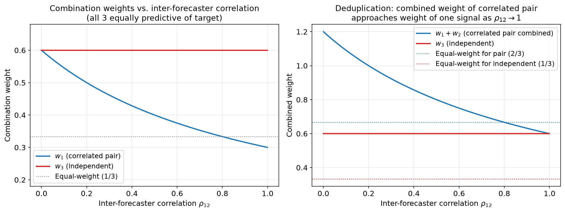
The key object is $\Sigma_{xx}^{-1}$: it downweights redundant signals. Suppose two forecasts are almost identical and a third forecast is independent. If all three are equally predictive of the target, $\Sigma_{xx}^{-1}$ gives the two redundant forecasts roughly half weight each, while the independent forecast keeps its full weight. Equal-weighting misses this distinction.
Vine copulas for outcome-forecast dependence
The Gaussian copula is restrictive: dependence is symmetric and linear in probit space. A vine copula replaces this with a product of bivariate pair copulas. With a C-vine rooted at the target,
\[p(u_y, u_1,\ldots,u_D) \approx p(u_y)\prod_{k=1}^D c_k(u_y,u_k).\]The conditional mean becomes
\[\mathbb{E}[u_y \mid u_1,\ldots,u_D] = \frac{\int_0^1 u \prod_k c_k(u,u_k)\,du} {\int_0^1 \prod_k c_k(u,u_k)\,du}.\]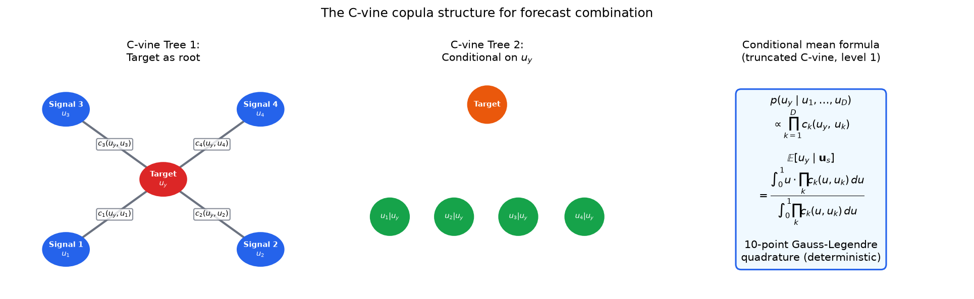
This one-dimensional integral can be evaluated by Gauss-Legendre quadrature. Each pair copula can be Gaussian, Student-t, Gumbel, Clayton, Frank, or a rotated version, selected by BIC. Here, a rotated version means a reflection of an asymmetric copula, useful for opposite-tail or negative dependence patterns.
Non-Gaussian pair copulas can help when a target-forecast relationship is not well described by a Gaussian copula. The figure below fixes Kendall $\tau$ at 0.5 for several bivariate copula families. They have the same overall rank association, but they transform the same signal rank into different expected outcome ranks, especially in the tails. A vine uses these pair copulas as building blocks inside a multivariate dependence model. The dotted diagonal is only an identity benchmark, $E[u_y\mid u_s]=u_s$: it maps a signal rank directly to the same outcome rank.
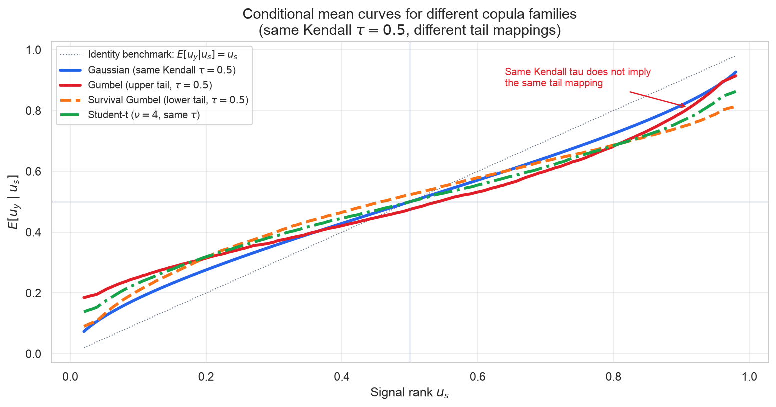
But the vine used here is deliberately simplified. A full vine over $(u_y,u_1,\ldots,u_D)$ would also model the dependence among the forecasts themselves, including conditional relationships such as forecast 1 versus forecast 2 after accounting for the target. That is more complete, but it requires many more pair-copulas and much more data.
The truncated target-rooted vine keeps only the target-signal links $c_k(u_y,u_k)$. In plain language, it asks: “how does each forecast relate to the realised outcome?” and then multiplies those pieces together. That multiplication quietly assumes that, once the realised outcome is known, the forecast signals are independent of each other. This is often false for SPF lead-time forecasts. If the nowcast and the one-quarter-ahead forecast both reflect the same public macro release, the truncated vine can count that same evidence twice. The Gaussian inverse $\Sigma_{xx}^{-1}$ corrects for redundancy directly; this truncated vine does not. This is not a limitation of vines in general: a fuller vine could add conditional signal-signal pair copulas and model that redundancy. The cost is statistical, because those extra pair copulas consume data. The trade-off here is therefore specific to the truncated approximation: it is attractive for nonlinear target-signal shapes when the signals themselves are not too redundant; otherwise the Gaussian copula’s analytical inter-signal correction is often more reliable in small macro samples.
Approach 2: forecast-error dependence
The second approach models errors directly. Write
\[X_k = Y + E_k.\]If the forecast-error vector is Gaussian and centred,
\[E = (E_1,\ldots,E_D)^\top \sim \mathcal{N}(0,\Sigma_E),\]then, for a candidate value $y$, the implied error vector is
\[e(y) = x - y\mathbf{1}.\]The log likelihood is, up to constants,
\[-\frac12 (x-y\mathbf{1})^\top \Sigma_E^{-1}(x-y\mathbf{1}).\]Maximising this over $y$ gives
\[\hat y = \frac{\mathbf{1}^\top \Sigma_E^{-1}x} {\mathbf{1}^\top \Sigma_E^{-1}\mathbf{1}}.\]This is the precision-weighted forecast combination.
Why call it Error GLS? GLS stands for generalized least squares. The analogy refers specifically to the inverse covariance of forecast errors. This is different from the outcome-side Gaussian copula above: there, $\Sigma_{xx}^{-1}$ is the inverse of the signal covariance matrix in probit-rank space. Here, $\Sigma_E^{-1}$ is the inverse of the forecast error covariance matrix in level space. Both inverses change the geometry of the combination problem so that redundant or noisy directions count less.
The covariance matrix is not the residual covariance from a regression of $y$ on $x$. It is the covariance of the forecasters’ errors with each other:
\[\Sigma_E = \operatorname{Cov}(E_1,\ldots,E_D).\]So Error GLS means: estimate how the forecasts err together, then combine the observed forecasts with weights implied by $\Sigma_E^{-1}$. If two forecasts usually make the same mistake, their shared error mode receives less weight. If one forecast has low error variance after accounting for the others, it receives more weight.
This is the approach that most deserves the GLS analogy because it is explicitly using the inverse covariance matrix of forecast errors. The zero-mean assumption is only for the clean derivation. In practice, one should either de-bias the forecast errors on the training sample or include an estimated mean error vector $\mu_E$; otherwise the method may combine forecasts precisely around the wrong centre.
It is also useful to compare the two inverse matrices that have appeared:
| Method | Inverse matrix | Space | What gets discounted? |
|---|---|---|---|
| Gaussian outcome copula | $\Sigma_{xx}^{-1}$ | probit-transformed forecast ranks | redundant signals |
| Error GLS | $\Sigma_E^{-1}$ | forecast errors in level space | redundant error modes |
The formulas look similar because both use a precision matrix, but they answer different probability questions. The outcome-side approach asks for the likely rank of $Y$ given the forecast ranks. The error-side approach asks which candidate $y$ makes the implied forecast errors most plausible.
The true copula-error generalisation
The Gaussian error model can be generalised with a copula. Let each error have marginal CDF $F_k$ and density $f_k$. Then
\[f_E(e_1,\ldots,e_D) = c(F_1(e_1),\ldots,F_D(e_D))\prod_k f_k(e_k).\]For each candidate $y$, compute implied errors
\[e_k(y)=x_k-y.\]Then choose
\[\hat y = \arg\max_y \left[ \log c(F_1(e_1(y)),\ldots,F_D(e_D(y))) + \sum_k \log f_k(e_k(y)) \right].\]This is the direct copula version of the “most plausible errors” idea. I estimate the marginal error distributions with KDE, transform candidate errors to error ranks, and fit either a Gaussian copula or a vine copula to those transformed errors. Prediction then becomes a one-dimensional optimisation over candidate $y$ values: choose the value whose implied transformed error vector has the highest fitted copula likelihood. In the experiments I use a robust grid search rather than a gradient method, because the KDE-plus-copula likelihood can be irregular in small samples.
This method is conceptually appealing, but it is more fragile than the closed-form Gaussian formula. It requires good marginal error estimates, enough data to fit the copula, and a stable optimisation for every prediction.
Synthetic checks
The synthetic studies below check whether the methods behave as theory says they should. For the outcome-side approach, Case A is a synthetic data-generating process with correlated Gaussian signals, where redundancy correction should help; Case B is a synthetic data-generating process with tail-dependent signals, where a vine has a real nonlinear dependence pattern to learn. For the error-side approach, I use one synthetic design with Gaussian correlated forecast errors and one with curved forecast-error dependence.
For the cross-sectional synthetic experiments, I report ICIR, the information coefficient ratio: the mean rank correlation between prediction and realised outcome, divided by its time-series standard deviation. The synthetic setup generates $T$ periods, each with $N$ cross-sectional observations; the information coefficient (IC) is the Spearman rank correlation between predicted and realised outcomes within each period. ICIR is then the mean IC divided by its standard deviation across the $T$ periods. Higher ICIR means the method is not only predictive on average, but predictably predictive through time.
Outcome-side approach: when Gaussian helps and when vine helps
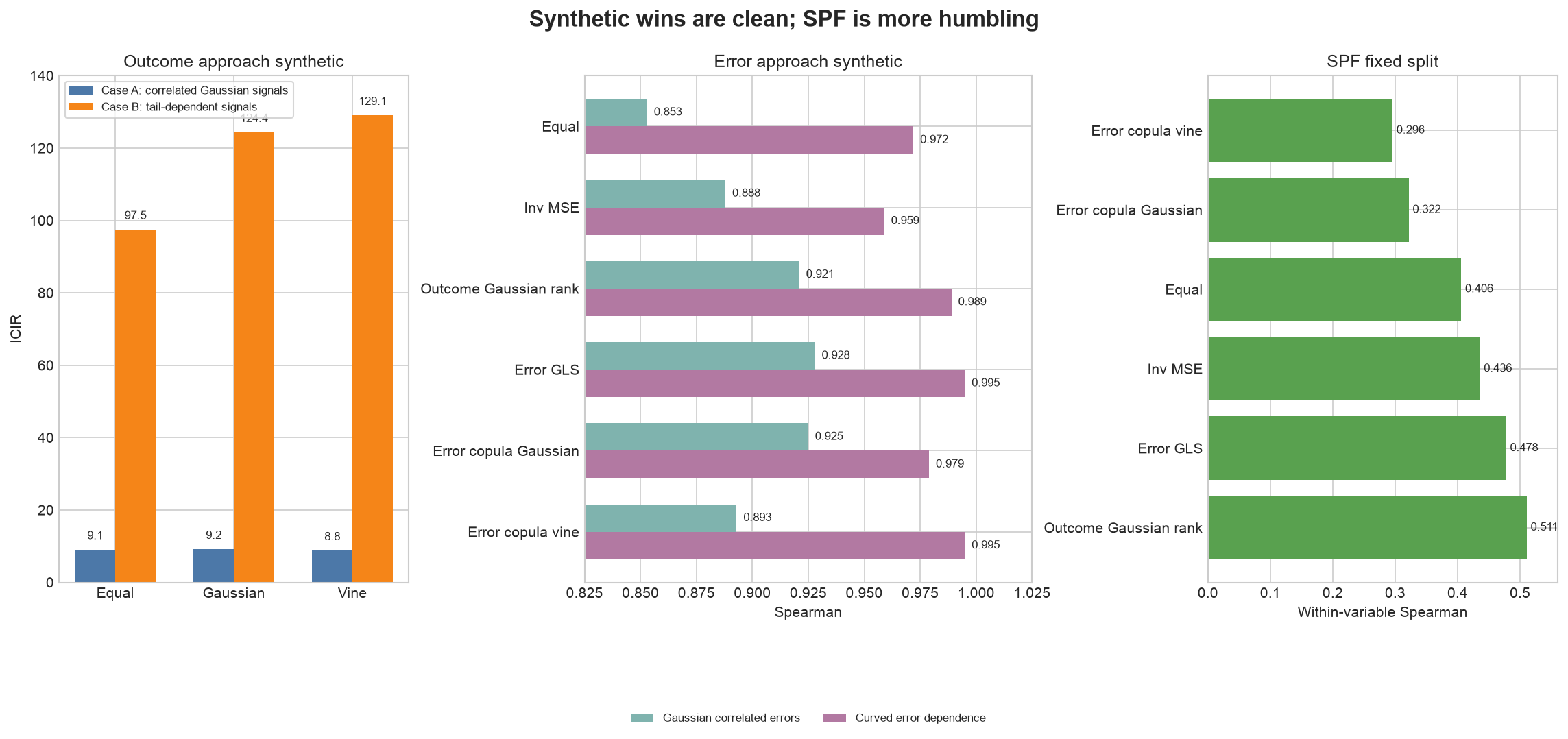
In the outcome-forecast synthetic study, Case A has correlated Gaussian signals. The Gaussian copula edges out equal-weight because $\Sigma_{xx}^{-1}$ deflates redundant signal clusters:
| Method | Case A ICIR |
|---|---|
| Equal-weight | 9.1 |
| Gaussian copula | 9.2 |
| Vine copula | 8.8 |
Case B has independent signals with non-Gaussian target-signal dependence: Gumbel upper-tail, survival Gumbel lower-tail, Student-t heavy tails, and Gaussian. The vine recovers the pair-copula families and wins:
| Method | Case B ICIR |
|---|---|
| Equal-weight | 97.5 |
| Gaussian copula | 124.4 |
| Vine copula | 129.1 |
The detailed synthetic comparison is shown below.
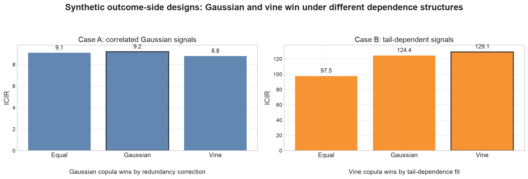
The synthetic example illustrates the intended role of the vine: it can improve on the Gaussian copula when the target-signal dependence is genuinely asymmetric, tail-dependent, or otherwise non-elliptical. That extra flexibility is useful only if the sample contains enough stable dependence signal to estimate it reliably. The empirical question is whether the SPF panel provides that much information.
Error-side approach: when GLS wins and when vine wins
In the error-dependence study, the Gaussian correlated-error case behaves as expected:
| Method | Spearman | RMSE |
|---|---|---|
| Equal-weight | 0.853 | 0.609 |
| Inverse MSE | 0.888 | 0.513 |
| Outcome Gaussian rank | 0.921 | 0.398 |
| Error GLS | 0.928 | 0.402 |
| Gaussian error-copula | 0.925 | 0.391 |
| Vine error-copula | 0.893 | 0.510 |
The RMSE for Outcome Gaussian rank is computed after mapping its predicted rank back through the empirical training distribution of the realised outcome. In this Gaussian-error design, the error covariance is the right summary of the error distribution. Error GLS therefore gives the best rank correlation, while the Gaussian error-copula gives the best level RMSE. The vine error-copula is more flexible, but that flexibility is unnecessary here and hurts out-of-sample performance.
But we can also construct a nonlinear error geometry where a covariance matrix is the wrong summary. Let a latent error factor $a$ drive
\[E_1 \approx a, \qquad E_2 \approx a^2 - 1, \qquad E_3 \approx -(a^2 - 1).\]The dependence is curved, not elliptical.
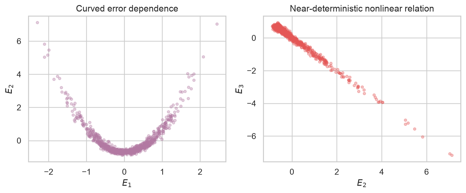
In that case the vine error-copula wins:
| Method | Spearman | RMSE |
|---|---|---|
| Equal-weight | 0.972 | 0.248 |
| Inverse MSE | 0.959 | 0.307 |
| Error GLS | 0.995 | 0.089 |
| Outcome Gaussian rank | 0.989 | 0.157 |
| Gaussian error-copula | 0.979 | 0.198 |
| Vine error-copula | 0.995 | 0.079 |
The RMSE for Outcome Gaussian rank is again computed after empirical rank-to-level calibration. It beats the Gaussian error-copula here because it directly models the target rank $Y \mid X_1,\ldots,X_D$, while the Gaussian error-copula is an indirect error-likelihood model and is misspecified for this curved error distribution. Error GLS also remains strong: although the dependence is nonlinear, $E_2$ and $E_3$ nearly cancel each other, so the covariance matrix still captures a powerful linear variance-reduction effect. The vine error-copula wins by using the remaining nonlinear error geometry that covariance compresses into an ellipse.
A humbling SPF fixed-split check
Synthetic data is useful because the data-generating process is known. The SPF panel is a harder test: the signal-to-noise ratio, the dependence structure, and the stability of the relationships are all uncertain.
Before the full rolling experiment of Part 3, I ran a simple fixed split on the SPF panel: train through 2010, test after 2010, requiring all five lead-time forecasts to be present. Each method is fitted separately by macro variable so that GDP growth, inflation, unemployment, housing, and industrial production are not forced onto one common scale. Rank/probit transforms, error KDEs, and covariance matrices are estimated on the training sample only. For evaluation, realised values and predictions are first converted to ranks within each macro variable; those within-variable ranks are then stacked, and one Spearman correlation is computed on the stacked rank data.
| Method | Spearman on stacked within-variable ranks |
|---|---|
| Outcome Gaussian rank | 0.511 |
| Error GLS | 0.478 |
| Inverse MSE | 0.436 |
| Equal-weight | 0.406 |
| Gaussian error-copula | 0.322 |
| Vine error-copula | 0.296 |
This first real-data check is humbling. The KDE plus copula-error likelihood underperforms here, which is consistent with a method that is too flexible for the available macro sample and for the stability of the train-test relationship. The outcome Gaussian rank model estimates one main object: a signal correlation matrix fitted to rank-transformed data. The error-copula approach estimates several objects in sequence: a KDE for each error marginal, then a multivariate copula fitted on the transformed error ranks. With only a few decades of quarterly observations, this two-stage estimation problem can add more variance than useful structure. Error GLS is less expressive, but it is also much lighter: it collapses the error dependence into a single parametric covariance matrix, which is why it holds up better in this check.
This is a useful caution for macroeconomic and financial forecasting: a flexible model can win in a synthetic design where its assumptions are true, but lose in real samples unless it is strongly regularised.
What Part 3 tests
Part 3 compares these method families on a walk-forward SPF horserace:
| Family | Method | What it tests |
|---|---|---|
| Baselines | Persistence, Lead 0, equal-weight, trimmed mean, inverse MSE | How far simple benchmarks go |
| Outcome-side approach | OLS on ranks, Gaussian copula on probit ranks, vine outcome copula | Whether modelling target-forecast dependence helps |
| Error-side approach | Error GLS, shrunk error GLS, Gaussian/vine error-copula | Whether modelling forecast-error dependence helps |
Part 3 will use a walk-forward evaluation with an expanding training window: the test date moves forward one forecast date at a time, and each fitted method is refitted using only the history available at that date. This is closer to actual forecast use than the fixed split above. It will also compare initial-release and latest-revised targets, and trace rolling out-of-sample performance through time. The named-forecaster experiment will remain separate, because same-horizon forecasters with similar skill are a different problem from cross-horizon signals with a structural lead-time hierarchy.
The key distinction is between two probability questions:
\[\mathbb{E}[Y \mid X_1,\ldots,X_D]\]versus
\[\arg\max_y f_E(X_1-y,\ldots,X_D-y).\]The first models the outcome conditional on the forecasts. The second models the joint forecast errors implied by a candidate outcome.
References and further reading
- Bates, J. M. and Granger, C. W. J. (1969), “The Combination of Forecasts”, Operational Research Quarterly.
- Granger, C. W. J. and Ramanathan, R. (1984), “Improved Methods of Combining Forecasts”, Journal of Forecasting.
- Genre, V., Kenny, G., Meyler, A. and Timmermann, A. (2013), “Combining Expert Forecasts: Can Anything Beat the Simple Average?”, International Journal of Forecasting.
- Sklar, A. (1959), “Fonctions de repartition a n dimensions et leurs marges,” Publications de l’Institut de Statistique de l’Universite de Paris.
- Bedford, T. and Cooke, R. M. (2002), “Vines: A New Graphical Model for Dependent Random Variables”, Annals of Statistics.
- Aas, K., Czado, C., Frigessi, A. and Bakken, H. (2009), “Pair-Copula Constructions of Multiple Dependence”, Insurance: Mathematics and Economics.