Performance attribution of a crypto market-neutral book on a statistical risk model
Performance attribution of a crypto market-neutral book on a statistical risk model
In this short blog post, we investigate whether a simple systematic market-neutral stat arb crypto book loads on the main components of a statistical risk model.
from datetime import timedelta
import pandas as pd
from tqdm import tqdm
import statsmodels.formula.api as smf
def compute_pnl_attribution(
    symbol,
    date,
    weights,
    returns,
    factor_returns,
    info,
    fexp_cols,
):
    if symbol not in info['symbol'].tolist():
        return {
            'date': date,
            'symbol': symbol,
            'ptf_weight': weights[symbol],
            'raw_pnl': 0,
            'factors_pnl': 0,
            'idio_pnl': 0,}

    factor_exposures = info[
        info['symbol'] == symbol][fexp_cols]
    factors_pnl = weights[symbol] * factor_exposures * factor_returns
    all_factors_pnl = factors_pnl.T.sum()
    raw_pnl = weights[symbol] * returns[symbol]
    idio_pnl = raw_pnl - all_factors_pnl

    output = {
        'date': date,
        'symbol': symbol,
        'ptf_weight': weights[symbol],
        'raw_pnl': float(raw_pnl),
        'factors_pnl': float(all_factors_pnl),
        'idio_pnl': float(idio_pnl),
    }

    for fexp_col in fexp_cols:
        output[f'{fexp_col}_pnl'] = float(factors_pnl[fexp_col])

    return output


def get_returns():
    prices = pd.read_parquet('../market_data/futures_prices.parquet')
    rect_prices = (prices
                   .pivot(index='close_time',
                          columns='symbol',
                          values='close')
                   .astype(float))
    return rect_prices.pct_change()


returns = get_returns()
returns.index = returns.index.normalize()
weights = pd.read_parquet(
    '../weights/histo_market_neutral_weights.parquet')
weights.index = weights.index.normalize()
dates = [str(date.date())
         for date in pd.date_range('2021-01-01', '2023-02-25')]
fexp_cols = ['v0', 'v1', 'v2', 'v3', 'v4']
all_attribs = []
for date in tqdm(dates):
    try:
        risk_model = pd.read_parquet(
            f'../stat_risk_models/{date[:4]}/{date[5:7]}/{date}_risk_model.parquet')
        date_weights = weights.loc[date].dropna()
        next_date = str((pd.to_datetime(date) + timedelta(days=1)).date())
        date_returns = returns.loc[next_date].fillna(0)
        crets = date_returns.reset_index()
        crets.columns = ['symbol', 'coin_return']
        info = pd.merge(crets, risk_model, on=['symbol'], how='outer')
        for col in [f'v{i}'for i in range(5)]:
            msk = info[col].isnull()
            info.loc[msk, col] = info.loc[~msk, col].mean()
        formula = 'coin_return' + '~' + (' + ').join(fexp_cols)
        model = smf.ols(formula=formula, data=info)
        res = model.fit()
        factor_returns = res.params[fexp_cols]

        attribs = []
        for symbol in date_weights.index.tolist():
            try:
                attribs.append(
                    compute_pnl_attribution(
                        symbol, date, date_weights, date_returns,
                        factor_returns, info, fexp_cols))
            except Exception as e:
                print(e)
                continue
    except Exception as e:
        print(e)
        continue

    all_attribs.append(pd.DataFrame(attribs))
100%|█████████████████████████████████████████| 786/786 [00:59<00:00, 13.30it/s]
attribs = pd.concat(all_attribs)
attribs['date'] = pd.to_datetime(attribs['date'])
attribs
| date | symbol | ptf_weight | raw_pnl | factors_pnl | idio_pnl | v0_pnl | v1_pnl | v2_pnl | v3_pnl | v4_pnl | |
|---|---|---|---|---|---|---|---|---|---|---|---|
| 0 | 2021-01-01 | ADAUSDT | 1.175635e-02 | 1.624158e-04 | 3.185707e-04 | -1.561549e-04 | -1.391260e-04 | 2.227900e-04 | 5.023173e-05 | 9.074977e-05 | 9.392519e-05 |
| 1 | 2021-01-01 | ALGOUSDT | 6.801738e-03 | 1.586560e-04 | -1.718120e-04 | 3.304680e-04 | -8.014604e-05 | -9.675818e-05 | -6.522148e-05 | 5.288577e-05 | 1.742793e-05 |
| 2 | 2021-01-01 | ATOMUSDT | -7.521109e-03 | 5.673168e-04 | 4.252014e-05 | 5.247966e-04 | 9.040750e-05 | -3.099810e-05 | 1.119393e-05 | -1.242631e-06 | -2.684055e-05 |
| 3 | 2021-01-01 | AVAXUSDT | -1.539033e-02 | 6.279792e-04 | -6.953236e-05 | 6.975116e-04 | 1.631459e-04 | 2.065687e-04 | -1.992583e-05 | -4.122042e-04 | -7.117004e-06 |
| 4 | 2021-01-01 | BALUSDT | -5.050539e-03 | -2.813499e-04 | 1.474914e-04 | -4.288413e-04 | 5.775383e-05 | 6.413726e-05 | 2.878981e-05 | 6.430396e-05 | -6.749351e-05 |
| ... | ... | ... | ... | ... | ... | ... | ... | ... | ... | ... | ... |
| 149 | 2023-02-25 | YFIUSDT | 1.007613e-06 | 5.159014e-08 | -3.263305e-08 | 8.422319e-08 | -3.366475e-08 | 7.640497e-11 | -4.932267e-10 | 9.126111e-10 | 5.359124e-10 |
| 150 | 2023-02-25 | ZECUSDT | 6.894340e-07 | 1.007718e-08 | -2.136069e-08 | 3.143787e-08 | -2.246475e-08 | 7.855229e-12 | -3.615739e-10 | 6.187657e-10 | 8.390088e-10 |
| 151 | 2023-02-25 | ZENUSDT | 9.939978e-07 | 3.087496e-08 | -3.529002e-08 | 6.616498e-08 | -3.593333e-08 | -2.607978e-10 | 8.432909e-11 | 2.446094e-10 | 5.751693e-10 |
| 152 | 2023-02-25 | ZILUSDT | 1.025030e-06 | 2.956200e-08 | -3.243898e-08 | 6.200099e-08 | -2.755038e-08 | 9.221657e-10 | -5.881167e-09 | -2.628073e-10 | 3.332073e-10 |
| 153 | 2023-02-25 | ZRXUSDT | 6.183873e-07 | -7.269799e-09 | -2.163312e-08 | 1.436332e-08 | -2.016682e-08 | 2.777037e-10 | -2.164615e-09 | 2.338815e-10 | 1.867287e-10 |
96845 rows × 11 columns
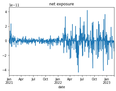
We check that the portfolio is indeed (dollar) market-neutral:
attribs.groupby('date')['ptf_weight'].sum().plot(title='net exposure');
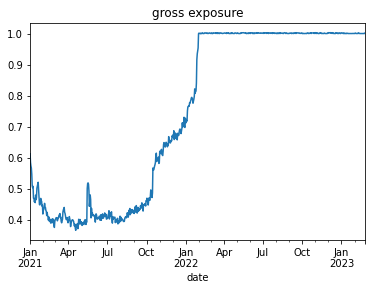
The portfolio is unlevered (max leverage = 1):
attribs.groupby('date')['ptf_weight'].apply(lambda x: sum(abs(x))).plot(title='gross exposure');
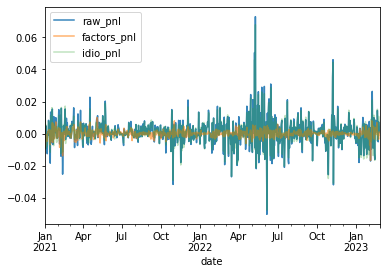
Time series of the daily returns of the portfolio (raw_pnl), the idiosyncratic component (idio_pnl), and the pnl coming from the statistical risk factors (factors_pnl):
pnl_types = ['raw_pnl', 'factors_pnl', 'idio_pnl']
for i, pnl_type in enumerate(pnl_types):
    attribs.groupby('date')[pnl_type].sum().plot(
        label=pnl_type, legend=True, alpha=0.3 * (3 - i))
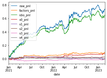
Cumulated pnl over the history:
for pnl_type in pnl_types:
    attribs.groupby('date')[pnl_type].sum().cumsum().plot(
        label=pnl_type, legend=True)
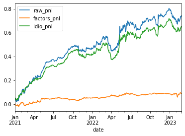
We can see that the risk factors are not contributing much to the total pnl. We are essentially orthogonal to these risk factors, and thus capturing ‘pure’ alpha (with respect to this statistical risk model). Note that this statistical risk model was not used to build the portfolio: It is an additional check to understand the source of alpha.
We can zoom in the individual risk components:
for pnl_type in pnl_types:
    attribs.groupby('date')[pnl_type].sum().cumsum().plot(
        label=pnl_type, legend=True)
for pnl_type in fexp_cols:
    attribs.groupby('date')[f'{pnl_type}_pnl'].sum().cumsum().plot(
        label=f'{pnl_type}_pnl', legend=True)
Considering only the risk factors pnl:
for pnl_type in fexp_cols:
    attribs.groupby('date')[f'{pnl_type}_pnl'].sum().cumsum().plot(
        label=f'{pnl_type}_pnl', legend=True)
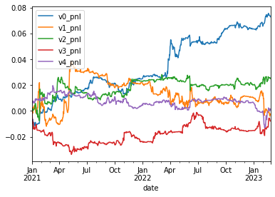
We can observe that the portfolio is earning money, with a good sharpe, from its small exposure to the main statistical risk factor v0. Check this previous blog for an interpretation of v0.
Let’s display the sharpe ratios for the different pnls:
for pnl_type in pnl_types:
    rets = attribs.groupby('date')[pnl_type].sum()
    sharpe = rets.mean() * 365**0.5 / rets.std()
    print(f"sharpe {pnl_type:>15}:{round(sharpe, 1):>10}")
for pnl_type in fexp_cols:
    rets = attribs.groupby('date')[f'{pnl_type}_pnl'].sum()
    sharpe = rets.mean() * 365**0.5 / rets.std()
    print(f"sharpe {f'{pnl_type}_pnl':>15}:{round(sharpe, 1):>10}")
sharpe         raw_pnl:       2.1
sharpe     factors_pnl:       0.9
sharpe        idio_pnl:       2.0
sharpe          v0_pnl:       1.7
sharpe          v1_pnl:      -0.0
sharpe          v2_pnl:       0.5
sharpe          v3_pnl:      -0.2
sharpe          v4_pnl:       0.0
The idiosyncratic component has a sharpe ratio close to the total pnl. It gets a small boost from being exposed to v0, but overall the risk factors contribution is small.
percentage_idio = (
    attribs.groupby('date')['idio_pnl'].sum().cumsum().iloc[-1] /
    attribs.groupby('date')['raw_pnl'].sum().cumsum().iloc[-1])
print(f"percentage of idiosyncratic pnl: " +
      f"{round(100 * percentage_idio)}%")
percentage of idiosyncratic pnl: 88%
Close to 90% of the pnl comes from the idiosyncratic component: Our signals are ‘pure’ alpha.
for pnl_type in pnl_types:
    total_pnl = attribs.groupby('date')[pnl_type].sum().cumsum().iloc[-1]
    print(f"total pnl {pnl_type:>12}:{round(100 * total_pnl):>10}%")
total pnl      raw_pnl:        74%
total pnl  factors_pnl:         9%
total pnl     idio_pnl:        65%
Conclusion: We checked that a simple market-neutral crypto portfolio is not exposed to the main risk factors (as seen by a statistical risk model). We could try to extend this study to fundamental risk factors, similarly to what is done in equities (check this book), but what are those factors???
Most likely, the alphas of today will become the betas (risk factors) of tomorrow.
Still early days…