First eigenvector correlation cryptos

Crypto PCA First Eigenvector

This short blog to illustrate an interesting fact that I found in An Analysis of Eigenvectors of a Stock Market Cross-Correlation Matrix by Nguyen and co-authors: The first eigenvector is not THE market portfolio (market-cap or uniformly weighted) as people usually believe, but a correlation-weighted market portfolio.

import numpy as np
import pandas as pd
from scipy.stats import rankdata

import matplotlib.pyplot as plt

def get_returns():
    """Compute daily returns from prices."""
    prices = pd.read_parquet('market_data/futures_prices.parquet')
    rect_prices = (prices
                   .pivot(index='close_time',
                          columns='symbol',
                          values='close')
                   .astype(float))
    
    return rect_prices.pct_change()

returns = get_returns()
xxx = returns.describe().T
coins = xxx[xxx['count'] > 500].index
returns = returns[coins].iloc[-500:]
returns.shape

(500, 101)

corr = returns.corr()
tri_a, tri_b = np.triu_indices(len(corr), k=1)
flat_corr = corr.values[tri_a, tri_b]
plt.hist(flat_corr, bins=100)
plt.axvline(flat_corr.mean(), color='k')
plt.show()

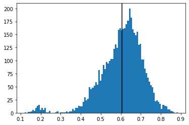
Distribution of correlations between cryptos returns

The average correlation between cryptos is quite high: 60%.

Let’s get the first eigenvector, and look into it:

eigenvals, eigenvecs = np.linalg.eig(corr)
idx = eigenvals.argsort()[::-1]   
pca_eigenvecs = eigenvecs[:, idx]

Distribution of the first eigenvector coefficients:

plt.hist(pca_eigenvecs[:, 0])
plt.show()

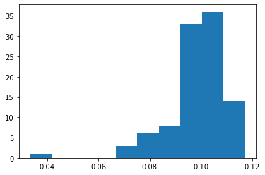
Distribution of the first eigenvector coefficients: All positive.

All positive.

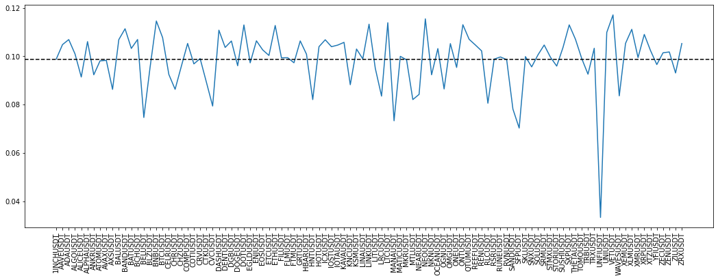
The first eigenvector:

plt.figure(figsize=(18, 6))
plt.plot(pca_eigenvecs[:, 0])
plt.axhline(np.mean(pca_eigenvecs[:, 0]), color='k', linestyle='--')
plt.xticks(range(len(returns.columns)), returns.columns, rotation=90)
plt.show()

It is a widespread belief that coefficients should be roughly uniformly distributed.

The first eigenvector. It is a widespread belief that coefficients should be roughly uniformly distributed.

Let’s define the ‘correlation weights’ as $w_i = \sum_{j=1}^n \rho_{ij}$.

corr_weight = corr.sum(axis=1)

corr_weight.sort_values()

symbol
UNFIUSDT    21.495413
SFPUSDT     43.984479
MANAUSDT    45.965002
BELUSDT     46.941996
SANDUSDT    49.003187
              ...    
LINKUSDT    70.467031
LTCUSDT     70.753819
BNBUSDT     71.275130
NEOUSDT     71.753468
VETUSDT     72.800973
Length: 101, dtype: float64

VET is the most correlated with the rest of the coins; UNFI the least.

normalized_weights = sum(pca_eigenvecs[:, 0]) * corr_weight / corr_weight.sum()

normalized_weights.sum(), sum(pca_eigenvecs[:, 0])

(9.980197180593267, 9.980197180593267)

plt.figure(figsize=(10, 4))
plt.subplot(1, 2, 1)
plt.scatter(normalized_weights, pca_eigenvecs[:, 0])
plt.subplot(1, 2, 2)
plt.scatter(rankdata(normalized_weights),
            rankdata(pca_eigenvecs[:, 0]));
plt.show()

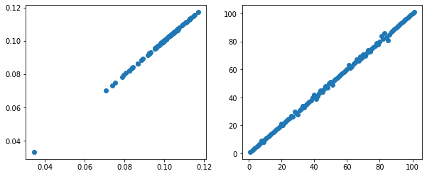
Correlation weights are the same as the first eigenvector coefficients (up to a rescaling, and a sign change)

On the above graphs, we can clearly see that the first eigenvector gives the same weights as the ‘correlation weights’ which are basically proportional to how much an asset (here a crypto) is correlated to the rest of the assets (cryptos) of the universe. The higher the correlation with the rest of the coins, the higher the weight.

In the paper An Analysis of Eigenvectors of a Stock Market Cross-Correlation Matrix, this observation is presented as an empirical fact verified on the Vietnamese stock market. In this blog, we have verified that this fact holds for cryptocurrencies as well. However, given its regularity and the intuitive relationship between average correlation and total variance, I am not sure this is purely an empirical fact: It may be possible to prove it.