Naive modelling of credit defaults using a Markov Random Field
Naive modelling of credit defaults using a Markov Random Field
Mid-2020, I read a book on probabilistic graphical models (PGMs) applied in finance by Alexander Denev.
Mid-2021, I hosted a machine learning meetup with an application of PGMs to predict the future states of economic and financial variables, and geopolitical events based on forward-looking views expressed by experts in news articles.
In this blog post, I finally provide some basic code to illustrate how they work in practice.
The model is very simple and loosely inspired by the paper Graphical Models for Correlated Defaults.
Three sectors co-dependent in their stress state are modelled: (finance, energy, retail). For each of these sectors, we consider a universe of three issuers.
Within Finance:
- Deutsche Bank
- Metro Bank
- Barclays
Within Energy:
- EDF
- Petrobras
- EnQuest
Within Retail:
- New Look
- Matalan
- Marks & Spencer
The probability of default of these issuers is partly idiosyncratic and partly depending on the stress within their respective sectors. Some distressed names such as New Look can have a high marginal probability of default, so high that the state of their sector (normal or stressed) does not matter much. Some other high-yield risky names such as Petrobras may strongly depend on how the whole energy sector is doing. On the other hand, a company such as EDF should be quite robust, and would require a very acute and persistent sector stress to move its default probability significantly higher.
We can encode this basic knowledge in terms of potentials:
+--------+-----------+-------------------+
| EDF    | energy    |   phi(EDF,energy) |
+========+===========+===================+
| EDF(0) | energy(0) |           90.0000 |
+--------+-----------+-------------------+
| EDF(0) | energy(1) |           80.0000 |
+--------+-----------+-------------------+
| EDF(1) | energy(0) |            5.0000 |
+--------+-----------+-------------------+
| EDF(1) | energy(1) |           40.0000 |
+--------+-----------+-------------------+
Conventions:
For a sector:
- 0: no-stress
- 1: under stress
For an issuer:
- 0: no-default
- 1: default
The choice of these potentials is not an easy task; It can be driven by historical fundamental or statistical relationships or forward-looking views.
Given a network structure, and a set of potentials, one can mechanically do inference using the pgmpy library.
We will show how to obtain a distribution of the number of defaults (and the expected number of defaults), a distribution of the losses (and the expected loss). From the joint probability table, we could also extract the default correlation.
tl;dr We use the library pgmpy to illustrate, on a toy example, how one can use a Markov Random Field (MRF) for modelling the distribution of defaults and losses in a credit portfolio.
The library pgmpy allows a user to encode a probabilistic graphical model (PGM) in a networkx compatible object; The library contains exact and approximate inference algorithms.
Building accurate PGM/MRF models require expert knowledge for considering a relevant graph structure, and attributing useful potentials.
import numpy as np
import pandas as pd
import networkx as nx

from pgmpy.models import MarkovNetwork
from pgmpy.factors.discrete import DiscreteFactor
from pgmpy.inference import BeliefPropagation
mm = MarkovNetwork()

# sectors are tied together
mm.add_edges_from([('finance', 'energy'),
                   ('finance', 'retail'),
                   ('energy', 'retail')])

# potentials between sectors
factor_1 = DiscreteFactor(
    variables=['finance', 'energy'],
    cardinality=[2, 2],
    values=[[90, 60],
            [70, 10]])

factor_2 = DiscreteFactor(
    variables=['finance', 'retail'],
    cardinality=[2, 2],
    values=[[80, 30],
            [10, 80]])

factor_3 = DiscreteFactor(
    variables=['energy', 'retail'],
    cardinality=[2, 2],
    values=[[60, 70],
            [5, 95]])

# issuers are dependent on their respective sectors
# given the sector, issuers are independent

# finance sector
mm.add_edges_from([('Deutsche Bank', 'finance'),
                   ('Metro Bank', 'finance'),
                   ('Barclays', 'finance')])

# potentials between issuer and its sector
factor_4 = DiscreteFactor(
    variables=['Deutsche Bank', 'finance'],
    cardinality=[2, 2],
    values=[[90, 10],
            [30, 60]])

factor_5 = DiscreteFactor(
    variables=['Metro Bank', 'finance'],
    cardinality=[2, 2],
    values=[[80, 5],
            [40, 60]])

factor_6 = DiscreteFactor(
    variables=['Barclays', 'finance'],
    cardinality=[2, 2],
    values=[[90, 20],
            [20, 50]])

# energy sector
mm.add_edges_from([('EDF', 'energy'),
                   ('Petrobras', 'energy'),
                   ('EnQuest', 'energy')])

# potentials between issuer and its sector
factor_7 = DiscreteFactor(
    variables=['EDF', 'energy'],
    cardinality=[2, 2],
    values=[[90, 80],
            [5, 40]])

factor_8 = DiscreteFactor(
    variables=['Petrobras', 'energy'],
    cardinality=[2, 2],
    values=[[60, 5],
            [50, 60]])

factor_9 = DiscreteFactor(
    variables=['EnQuest', 'energy'],
    cardinality=[2, 2],
    values=[[80, 10],
            [20, 50]])

# retail sector
mm.add_edges_from([('New Look', 'retail'),
                   ('Matalan', 'retail'),
                   ('Marks & Spencer', 'retail')])

# potentials between issuer and its sector
factor_10 = DiscreteFactor(
    variables=['New Look', 'retail'],
    cardinality=[2, 2],
    values=[[5, 2],
            [60, 90]])

factor_11 = DiscreteFactor(
    variables=['Matalan', 'retail'],
    cardinality=[2, 2],
    values=[[40, 20],
            [30, 70]])

factor_12 = DiscreteFactor(
    variables=['Marks & Spencer', 'retail'],
    cardinality=[2, 2],
    values=[[80, 30],
            [10, 50]])

mm.add_factors(factor_1, factor_2, factor_3,
               factor_4, factor_5, factor_6,
               factor_7, factor_8, factor_9,
               factor_10, factor_11, factor_12)
nx.draw_planar(mm, with_labels=True, node_size=1000, node_shape='h',
               node_color=['orange', 'orange', 'orange',
                           '#1f78b4', '#1f78b4', '#1f78b4',
                           '#1f78b4', '#1f78b4', '#1f78b4',
                           '#1f78b4', '#1f78b4', '#1f78b4',],
              edge_color=['purple', 'purple', 'k',
                          'k', 'k', 'purple',
                          'k', 'k', 'k',
                          'k', 'k', 'k',])
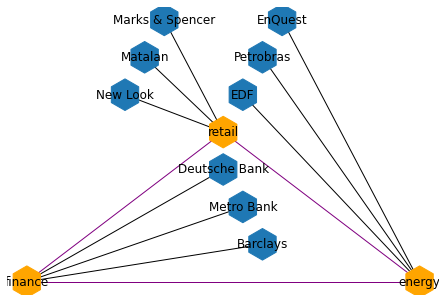
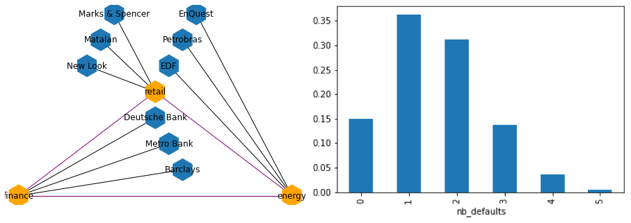
Markov Random Field (MRF) between sectors and issuers
A few examples of inference using this MRF
Example 1
# inference
belief_propagation = BeliefPropagation(mm)
r = belief_propagation.query(variables=['EDF'], evidence={'energy': 0})
Given that we observe that the energy sector is not under stress, EDF has only a 5% chance of defaulting. Note that, at the time of writing this blog post, EDF CDS-implied probability (in the Q-world) of defaulting within 5 years is 5.5%
… but this is totally coincidental as I did not calibrate the potentials.
print(r)
+--------+------------+
| EDF    |   phi(EDF) |
+========+============+
| EDF(0) |     0.9474 |
+--------+------------+
| EDF(1) |     0.0526 |
+--------+------------+
Example 2
# inference
belief_propagation = BeliefPropagation(mm)
r = belief_propagation.query(variables=['EDF'], evidence={})
If we cannot observe the state of the energy sector, then EDF has a higher chance of defaulting (9%) as it is possible that the energy sector is under stress.
print(r)
+--------+------------+
| EDF    |   phi(EDF) |
+========+============+
| EDF(0) |     0.9072 |
+--------+------------+
| EDF(1) |     0.0928 |
+--------+------------+
Example 3
# inference
belief_propagation = BeliefPropagation(mm)
r = belief_propagation.query(variables=['New Look'],
                             evidence={'Marks & Spencer': 1})
Given that Marks & Spencer (a much safer name) has defaulted, New Look has now an increased chance of defaulting: 97%.
print(r)
+-------------+-----------------+
| New Look    |   phi(New Look) |
+=============+=================+
| New Look(0) |          0.0286 |
+-------------+-----------------+
| New Look(1) |          0.9714 |
+-------------+-----------------+
Example 4
# inference
belief_propagation = BeliefPropagation(mm)
r = belief_propagation.query(variables=['New Look'],
                             evidence={'retail': 0})
Even if the retail sector is doing ok, New Look is a distressed name with a high probability of default (92%).
print(r)
+-------------+-----------------+
| New Look    |   phi(New Look) |
+=============+=================+
| New Look(0) |          0.0769 |
+-------------+-----------------+
| New Look(1) |          0.9231 |
+-------------+-----------------+
Impact of defaults on a credit portfolio and the distribution of losses
Amongst the 9 available issuers, let’s consider the following portfolio containing bonds from these 5 issuers:
portfolio_names = ['EDF', 'Petrobras', 'EnQuest', 'Matalan', 'Barclays']
portfolio_exposures = [2e6, 400e3, 300e3, 600e3, 3e6]
LGD = 0.9

print('Total notional: USD', str(sum(portfolio_exposures) / 1e6) + 'MM')
Total notional: USD 6.3MM
We have a USD 6.3MM total exposure to these names (notional).
We assume that in case of default, we recover only 10% (LGD = 90%).
Let’s start using the model:
r = belief_propagation.query(variables=['finance', 'retail', 'energy'],
                             evidence={})
print(r)
+------------+-----------+-----------+------------------------------+
| finance    | retail    | energy    |   phi(finance,retail,energy) |
+============+===========+===========+==============================+
| finance(0) | retail(0) | energy(0) |                       0.4238 |
+------------+-----------+-----------+------------------------------+
| finance(0) | retail(0) | energy(1) |                       0.0105 |
+------------+-----------+-----------+------------------------------+
| finance(0) | retail(1) | energy(0) |                       0.2999 |
+------------+-----------+-----------+------------------------------+
| finance(0) | retail(1) | energy(1) |                       0.1215 |
+------------+-----------+-----------+------------------------------+
| finance(1) | retail(0) | energy(0) |                       0.0083 |
+------------+-----------+-----------+------------------------------+
| finance(1) | retail(0) | energy(1) |                       0.0000 |
+------------+-----------+-----------+------------------------------+
| finance(1) | retail(1) | energy(0) |                       0.1251 |
+------------+-----------+-----------+------------------------------+
| finance(1) | retail(1) | energy(1) |                       0.0109 |
+------------+-----------+-----------+------------------------------+
There is a 42% chance that no sector is under stress.
If we observe that the finance sector is doing ok, and that Marks & Spencer is still doing business as usual, then this is the current joint probabilities associated to the potential defaults in the portfolio:
r = belief_propagation.query(variables=portfolio_names,
                             evidence={'finance': 0,
                                       'Marks & Spencer': 0})
print(r)
+-------------+------------+--------------+------------+--------+-----------------------------------------------+
| Barclays    | EnQuest    | Petrobras    | Matalan    | EDF    |   phi(Barclays,EnQuest,Petrobras,Matalan,EDF) |
+=============+============+==============+============+========+===============================================+
| Barclays(0) | EnQuest(0) | Petrobras(0) | Matalan(0) | EDF(0) |                                        0.1495 |
+-------------+------------+--------------+------------+--------+-----------------------------------------------+
| Barclays(0) | EnQuest(0) | Petrobras(0) | Matalan(0) | EDF(1) |                                        0.0084 |
+-------------+------------+--------------+------------+--------+-----------------------------------------------+
| Barclays(0) | EnQuest(0) | Petrobras(0) | Matalan(1) | EDF(0) |                                        0.1552 |
+-------------+------------+--------------+------------+--------+-----------------------------------------------+
| Barclays(0) | EnQuest(0) | Petrobras(0) | Matalan(1) | EDF(1) |                                        0.0088 |
+-------------+------------+--------------+------------+--------+-----------------------------------------------+
| Barclays(0) | EnQuest(0) | Petrobras(1) | Matalan(0) | EDF(0) |                                        0.1268 |
+-------------+------------+--------------+------------+--------+-----------------------------------------------+
| Barclays(0) | EnQuest(0) | Petrobras(1) | Matalan(0) | EDF(1) |                                        0.0081 |
+-------------+------------+--------------+------------+--------+-----------------------------------------------+
| Barclays(0) | EnQuest(0) | Petrobras(1) | Matalan(1) | EDF(0) |                                        0.1350 |
+-------------+------------+--------------+------------+--------+-----------------------------------------------+
| Barclays(0) | EnQuest(0) | Petrobras(1) | Matalan(1) | EDF(1) |                                        0.0102 |
+-------------+------------+--------------+------------+--------+-----------------------------------------------+
| Barclays(0) | EnQuest(1) | Petrobras(0) | Matalan(0) | EDF(0) |                                        0.0383 |
+-------------+------------+--------------+------------+--------+-----------------------------------------------+
| Barclays(0) | EnQuest(1) | Petrobras(0) | Matalan(0) | EDF(1) |                                        0.0026 |
+-------------+------------+--------------+------------+--------+-----------------------------------------------+
| Barclays(0) | EnQuest(1) | Petrobras(0) | Matalan(1) | EDF(0) |                                        0.0412 |
+-------------+------------+--------------+------------+--------+-----------------------------------------------+
| Barclays(0) | EnQuest(1) | Petrobras(0) | Matalan(1) | EDF(1) |                                        0.0034 |
+-------------+------------+--------------+------------+--------+-----------------------------------------------+
| Barclays(0) | EnQuest(1) | Petrobras(1) | Matalan(0) | EDF(0) |                                        0.0431 |
+-------------+------------+--------------+------------+--------+-----------------------------------------------+
| Barclays(0) | EnQuest(1) | Petrobras(1) | Matalan(0) | EDF(1) |                                        0.0077 |
+-------------+------------+--------------+------------+--------+-----------------------------------------------+
| Barclays(0) | EnQuest(1) | Petrobras(1) | Matalan(1) | EDF(0) |                                        0.0627 |
+-------------+------------+--------------+------------+--------+-----------------------------------------------+
| Barclays(0) | EnQuest(1) | Petrobras(1) | Matalan(1) | EDF(1) |                                        0.0170 |
+-------------+------------+--------------+------------+--------+-----------------------------------------------+
| Barclays(1) | EnQuest(0) | Petrobras(0) | Matalan(0) | EDF(0) |                                        0.0332 |
+-------------+------------+--------------+------------+--------+-----------------------------------------------+
| Barclays(1) | EnQuest(0) | Petrobras(0) | Matalan(0) | EDF(1) |                                        0.0019 |
+-------------+------------+--------------+------------+--------+-----------------------------------------------+
| Barclays(1) | EnQuest(0) | Petrobras(0) | Matalan(1) | EDF(0) |                                        0.0345 |
+-------------+------------+--------------+------------+--------+-----------------------------------------------+
| Barclays(1) | EnQuest(0) | Petrobras(0) | Matalan(1) | EDF(1) |                                        0.0020 |
+-------------+------------+--------------+------------+--------+-----------------------------------------------+
| Barclays(1) | EnQuest(0) | Petrobras(1) | Matalan(0) | EDF(0) |                                        0.0282 |
+-------------+------------+--------------+------------+--------+-----------------------------------------------+
| Barclays(1) | EnQuest(0) | Petrobras(1) | Matalan(0) | EDF(1) |                                        0.0018 |
+-------------+------------+--------------+------------+--------+-----------------------------------------------+
| Barclays(1) | EnQuest(0) | Petrobras(1) | Matalan(1) | EDF(0) |                                        0.0300 |
+-------------+------------+--------------+------------+--------+-----------------------------------------------+
| Barclays(1) | EnQuest(0) | Petrobras(1) | Matalan(1) | EDF(1) |                                        0.0023 |
+-------------+------------+--------------+------------+--------+-----------------------------------------------+
| Barclays(1) | EnQuest(1) | Petrobras(0) | Matalan(0) | EDF(0) |                                        0.0085 |
+-------------+------------+--------------+------------+--------+-----------------------------------------------+
| Barclays(1) | EnQuest(1) | Petrobras(0) | Matalan(0) | EDF(1) |                                        0.0006 |
+-------------+------------+--------------+------------+--------+-----------------------------------------------+
| Barclays(1) | EnQuest(1) | Petrobras(0) | Matalan(1) | EDF(0) |                                        0.0092 |
+-------------+------------+--------------+------------+--------+-----------------------------------------------+
| Barclays(1) | EnQuest(1) | Petrobras(0) | Matalan(1) | EDF(1) |                                        0.0008 |
+-------------+------------+--------------+------------+--------+-----------------------------------------------+
| Barclays(1) | EnQuest(1) | Petrobras(1) | Matalan(0) | EDF(0) |                                        0.0096 |
+-------------+------------+--------------+------------+--------+-----------------------------------------------+
| Barclays(1) | EnQuest(1) | Petrobras(1) | Matalan(0) | EDF(1) |                                        0.0017 |
+-------------+------------+--------------+------------+--------+-----------------------------------------------+
| Barclays(1) | EnQuest(1) | Petrobras(1) | Matalan(1) | EDF(0) |                                        0.0139 |
+-------------+------------+--------------+------------+--------+-----------------------------------------------+
| Barclays(1) | EnQuest(1) | Petrobras(1) | Matalan(1) | EDF(1) |                                        0.0038 |
+-------------+------------+--------------+------------+--------+-----------------------------------------------+
jpt = []
for i in range(32):
    jpt.append([int(e) for e in ("{0:5b}"
                                 .format(i)
                                 .replace(' ', '0'))])
jpt = pd.DataFrame(jpt, columns=r.variables)
jpt['joint_probability'] = r.values.flatten()
jpt['joint_probability'].sum()
1.0
From the joint probability distribution displayed above, we can compute the distribution of the number of defaults:
jpt['nb_defaults'] = jpt[portfolio_names].sum(axis=1)
distribution_nb_defaults = (jpt
                            .groupby('nb_defaults')['joint_probability']
                            .sum())
distribution_nb_defaults.plot(kind='bar');
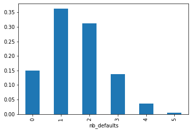
Distribution of the number of defaults in the portfolio
print('Expected number of defaults in the portfolio:',
      round(sum(distribution_nb_defaults.index *
                distribution_nb_defaults.values), 1))
Expected number of defaults in the portfolio: 1.6
Besides the expected number of defaults, the distribution of losses is even more informative:
exposures = pd.DataFrame(portfolio_exposures).T
exposures.columns = portfolio_names
exposures = exposures.reindex(index=jpt.index).ffill()
default_exposures = jpt[portfolio_names] * exposures * LGD
jpt['LGD'] = default_exposures.sum(axis=1)
expected_loss = (jpt['LGD'] * jpt['joint_probability']).sum()
print(f'Expected loss with respect to a par value of USD ' +
      f'{sum(portfolio_exposures)/1e6}MM ' +
      f'is USD {round(expected_loss / 1e6, 1)}MM.')

print(f'Expected loss: ' +
      f'{int(100 * round(expected_loss / sum(portfolio_exposures), 2))}% ' +
      f'of the notional.')
Expected loss with respect to a par value of USD 6.3MM is USD 1.2MM.
Expected loss: 19% of the notional.
jpt['loss_bucket'] = pd.qcut(jpt['LGD'], q=10)
jpt.groupby('loss_bucket')['joint_probability'].sum().plot(kind='bar');
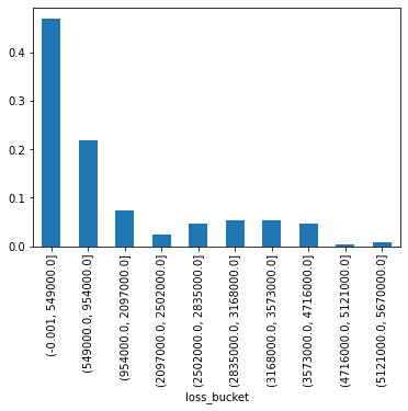
Distribution of losses with respect to par value
jpt.groupby('loss_bucket')['joint_probability'].sum().cumsum()
loss_bucket
(-0.001, 549000.0]        0.469960
(549000.0, 954000.0]      0.689263
(954000.0, 2097000.0]     0.762897
(2097000.0, 2502000.0]    0.787553
(2502000.0, 2835000.0]    0.834408
(2835000.0, 3168000.0]    0.888119
(3168000.0, 3573000.0]    0.941345
(3573000.0, 4716000.0]    0.987143
(4716000.0, 5121000.0]    0.991483
(5121000.0, 5670000.0]    1.000000
Name: joint_probability, dtype: float64