CopulaGAN (the 3d case) - A first naive attempt
CopulaGAN (the 3d case) - A first naive attempt
In this blog, we start the research effort around CopulaGAN.
The goal is to sample from a realistic dependence structure of $n$ variables (e.g. stocks returns, credit default swaps spreads changes).
Whereas CorrGAN is well suited to work with hundreds of variables, I hope that CopulaGAN will be able to scale to deal with the dozens of variables. However, CopulaGAN should be able to describe much more precisely the dependence structure of $n$ variables than a $n \times n$ correlation matrix generated by CorrGAN would since a correlation matrix discards a lot of information:
-
a correlation coefficient is a simplistic summary of a bivariate distribution between two variables,
-
only pairwise relationship between the variables is considered (though the PSD-ness of the matrix is enforcing some multivariate constraints).
Copulas, unlike correlation matrices, encode the whole dependence distribution.
We start exploring the possibility of sampling realistic vectors using GANs (or VAEs) from high-dimensional copulas by playing with a simple case: $d = 3$.
We follow the steps of the study we did earlier for CorrGAN in 3 dimensions.
TL;DR CopulaGAN 3D seems to approximately work using off-the-shelf GAN code. However, it has flaws, and won’t probably extend to higher dimensions (as it was the case for CorrGAN).
Like CorrGAN, CopulaGAN faces the permutation invariance problem. In the case of CorrGAN, we solved it by using a natural ordering of the data (cf. this blog for the permutation invariance discussion, and this blog for the ordering trick using hierarchical clustering). In the case of CopulaGAN, it is not clear what would be a proper ordering of the empirical measures… Stochastic Deep Networks offer a promising avenue to solve this issue.
%matplotlib inline

import pandas as pd
import numpy as np
from scipy.stats import rankdata
from numpy.random import seed
import tensorflow as tf
from mpl_toolkits.mplot3d import Axes3D
from matplotlib import animation
import matplotlib.pyplot as plt

seed(42)
The data loaded below was built by choosing 3 stocks among approximately 500, then ranking their returns (time series), and finally normalizing the ranks into $[0, 1]^3$. We end up with 3 uniform margins whose joint distribution is the empirical copula.
copulas = np.load('copulas-3d/copula_sample.npy')
copulas.shape
(897120, 3)
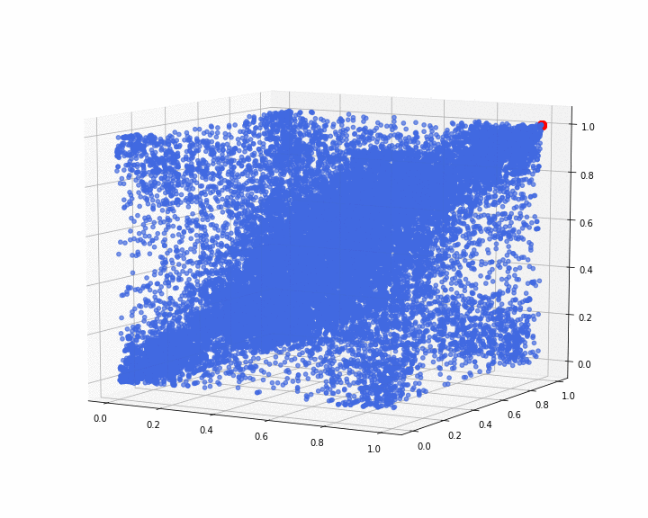
we display below what the 3d empirical copula looks like:
xs = copulas[:20000, 0]
ys = copulas[:20000, 1]
zs = copulas[:20000, 2]

fig = plt.figure(figsize=(10, 8))
ax = plt.axes(projection='3d')
ax.scatter(xs, ys, zs, color='royalblue', alpha=0.2)
ax.scatter(1, 1, 1, color='red', s=100)
ax.view_init(30, 45)
plt.tight_layout()
plt.show()
We can notice that the distribution is rather symmetric around the diagonal ((0,0,0), (1,1,1)).
The red dot is locating the point (1, 1, 1), and has no other meaning. It is just for visual convenience in the following animations.
def init():
    ax.scatter(xs, ys, zs, color='royalblue', alpha=0.2)
    ax.scatter(1, 1, 1, color='red', s=100)
    return fig,

def animate_mpg(i):
    if i < 90:
        ax.view_init(elev=10, azim=i*4)
    elif i < 180:
        ax.view_init(elev=10+2*(i%90), azim=(i%90)*4)
    else:
        ax.view_init(elev=190-2*(i%90), azim=0)
    return fig,

def animate_gif(i):
    if i < 90:
        ax.view_init(elev=10, azim=-60+i*4)
    elif i < 133:
        ax.view_init(elev=10+(i%90)*4, azim=-60)
    else:
        ax.view_init(elev=-180+(10+(i%90)*4)%180, azim=-60)
    return fig,
An animation of the 3d point cloud representing the copula:
fn = 'figs/empirical_copula_3d'

anim = animation.FuncAnimation(
    fig, animate_mpg, init_func=init, frames=270, interval=50,
    blit=True)

anim.save(fn + '.mp4', writer='ffmpeg', fps=1000 / 50)

anim = animation.FuncAnimation(
    fig, animate_gif, init_func=init, frames=180, interval=50,
    blit=True)

anim.save(fn + '.gif', writer='imagemagick', fps=1000 / 50)
We are now defining a basic GAN, whose goal is to sample 3d vectors from this distribution. We are using the basic code that got us started for CorrGAN first experiments:
def generator(Z, hsize=[64, 64, 16], reuse=False):
    with tf.variable_scope("GAN/Generator", reuse=reuse):
        h1 = tf.layers.dense(Z, hsize[0], activation=tf.nn.leaky_relu)
        h2 = tf.layers.dense(h1, hsize[1], activation=tf.nn.leaky_relu)
        h3 = tf.layers.dense(h2, hsize[2], activation=tf.nn.leaky_relu)
        out = tf.layers.dense(h3, 3)

    return out
def discriminator(X, hsize=[64, 64, 16], reuse=False):
    with tf.variable_scope("GAN/Discriminator", reuse=reuse):
        h1 = tf.layers.dense(X, hsize[0], activation=tf.nn.leaky_relu)
        h2 = tf.layers.dense(h1, hsize[1], activation=tf.nn.leaky_relu)
        h3 = tf.layers.dense(h2, hsize[2], activation=tf.nn.leaky_relu)
        h4 = tf.layers.dense(h3, 3)
        out = tf.layers.dense(h4, 1)

    return out, h4
X = tf.placeholder(tf.float32, [None, 3])
Z = tf.placeholder(tf.float32, [None, 3])
G_sample = generator(Z)
r_logits, r_rep = discriminator(X)
f_logits, g_rep = discriminator(G_sample, reuse=True)
disc_loss = tf.reduce_mean(
    tf.nn.sigmoid_cross_entropy_with_logits(
        logits=r_logits, labels=tf.ones_like(r_logits)) +
    tf.nn.sigmoid_cross_entropy_with_logits(
        logits=f_logits, labels=tf.zeros_like(f_logits)))

gen_loss = tf.reduce_mean(
    tf.nn.sigmoid_cross_entropy_with_logits(
        logits=f_logits, labels=tf.ones_like(f_logits)))
gen_vars = tf.get_collection(
    tf.GraphKeys.GLOBAL_VARIABLES, scope="GAN/Generator")
disc_vars = tf.get_collection(
    tf.GraphKeys.GLOBAL_VARIABLES, scope="GAN/Discriminator")

gen_step = tf.train.RMSPropOptimizer(
    learning_rate=0.0001).minimize(gen_loss, var_list=gen_vars)
disc_step = tf.train.RMSPropOptimizer(
    learning_rate=0.0001).minimize(disc_loss, var_list=disc_vars)
The GAN model is now defined.
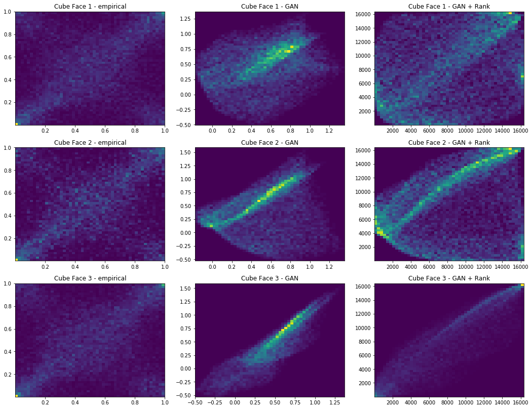
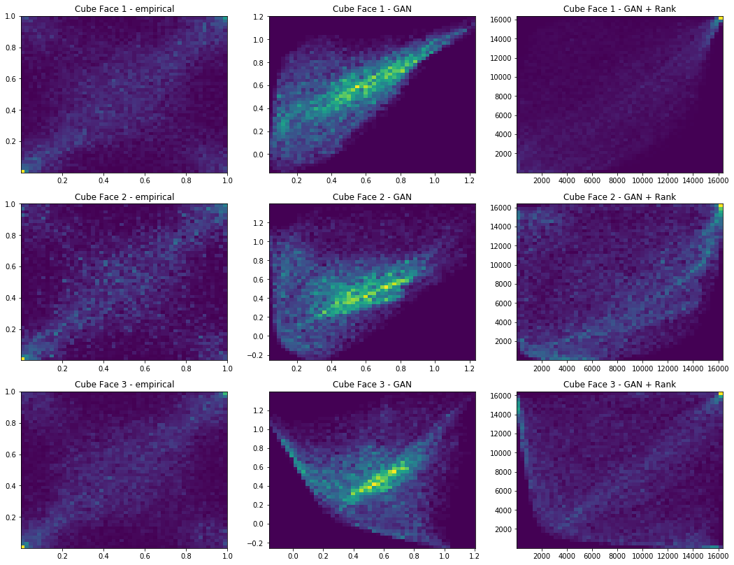
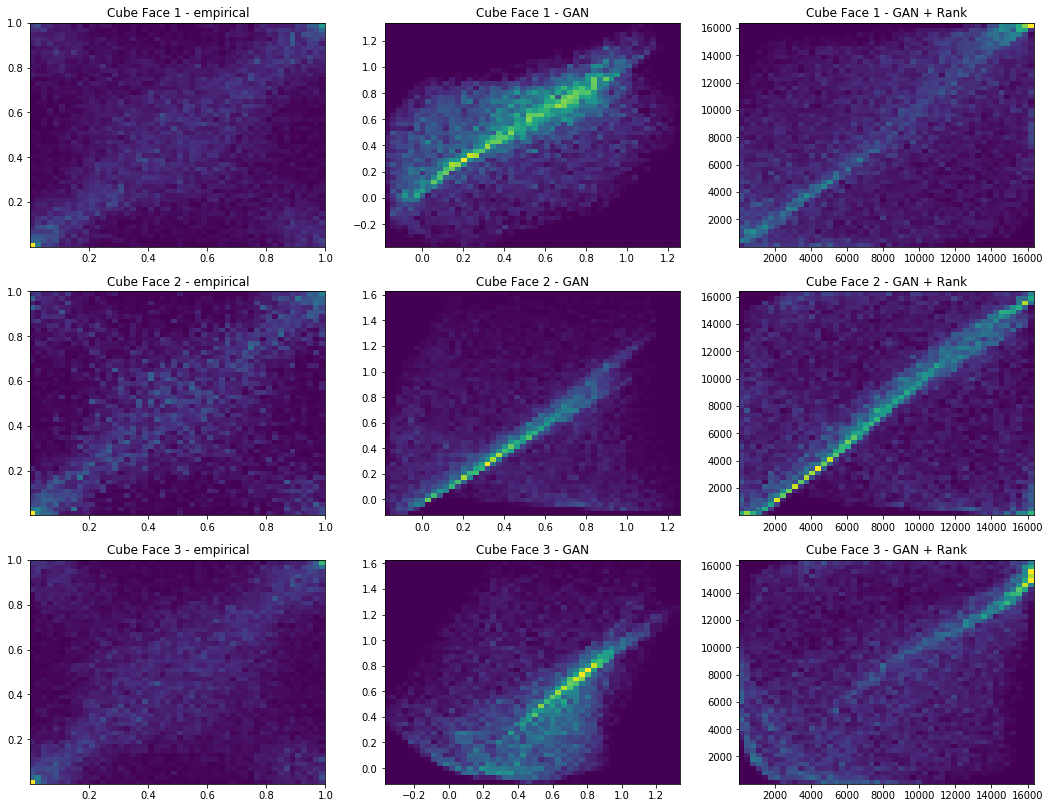
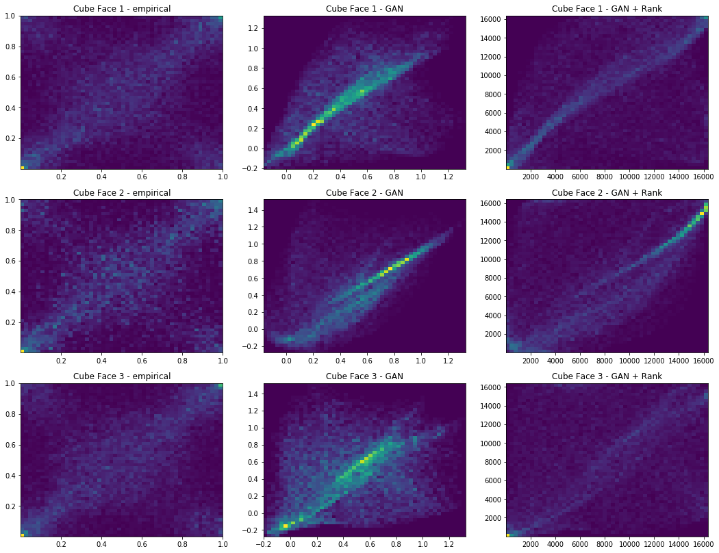
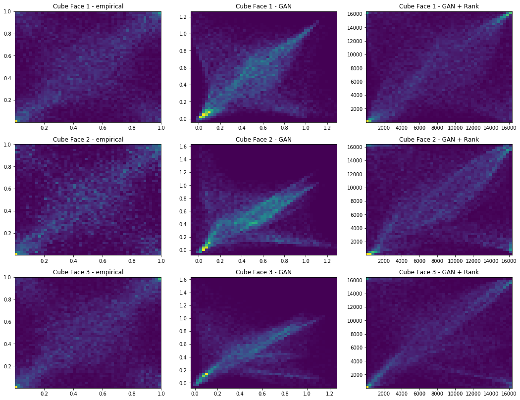
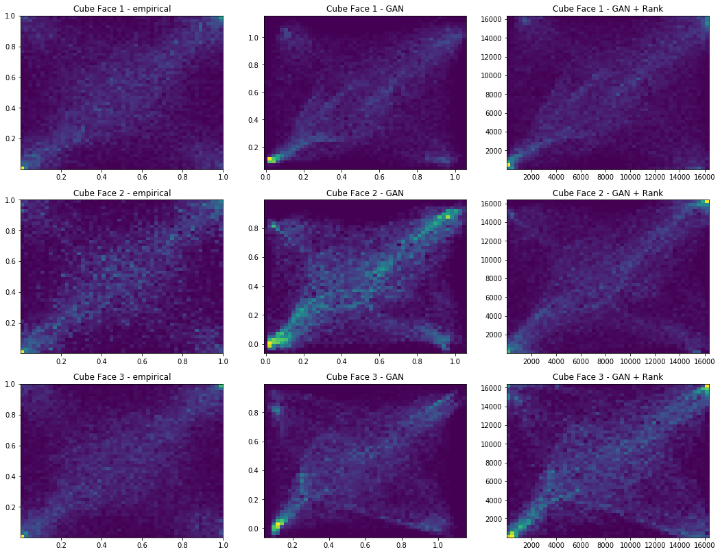
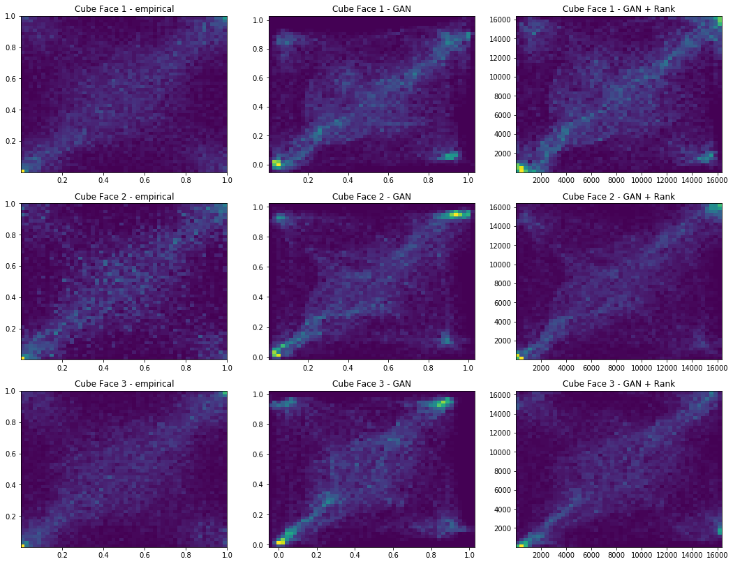
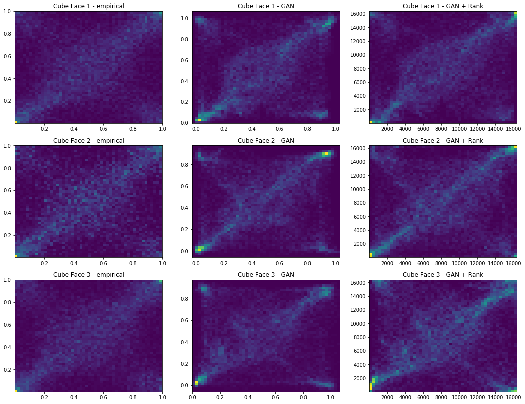
To monitor how the training goes, we will also look at the projections on the 2d faces of the unit cube $[0, 1]^3$, i.e. the empirical copulas of $(x_1, x_2)$, $(x_1, x_3)$, $(x_2, x_3)$.
def plot_faces(e_plot, g_plot):
    plt.figure(figsize=(18, 14))
    nb_bins = 50
    for count, (idx1, idx2) in enumerate([[0, 1], [0, 2], [1, 2]]):
        plt.subplot(3, 3, 3 * count + 1)
        plt.hist2d(e_plot[:, idx1], e_plot[:, idx2],
                   bins=nb_bins)
        plt.title('Cube Face {} - empirical'.format(count + 1))
        plt.subplot(3, 3, 3 * count + 2)
        plt.hist2d(g_plot[:, idx1], g_plot[:, idx2],
                   bins=nb_bins)
        plt.title('Cube Face {} - GAN'.format(count + 1))
        plt.subplot(3, 3, 3 * count + 3)
        plt.hist2d(rankdata(g_plot[:, idx1]), rankdata(g_plot[:, idx2]),
                   bins=nb_bins)
        plt.title('Cube Face {} - GAN + Rank'.format(count + 1))
    plt.show()
We will sample $2^{14} = 16384$ points for the display of the real empirical distribution, and the GAN generated one.
def sample_Z(m, n):
    return np.random.uniform(-1., 1., size=[m, n])

def sample_from_copula(n=10000):
    idx = [randint(0, len(copulas) - 1)
           for j in range(n)]

    return copulas[idx, :]

n_dots = 2**14
x_plot = sample_from_copula(n=n_dots)
Z_plot = sample_Z(n_dots, 3)
Batches contain 512 points.
sess = tf.Session()
tf.global_variables_initializer().run(session=sess)

batch_size = 2**9
nd_steps = 5
ng_steps = 5
And, finally, the main loop for training the GAN.
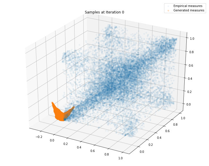
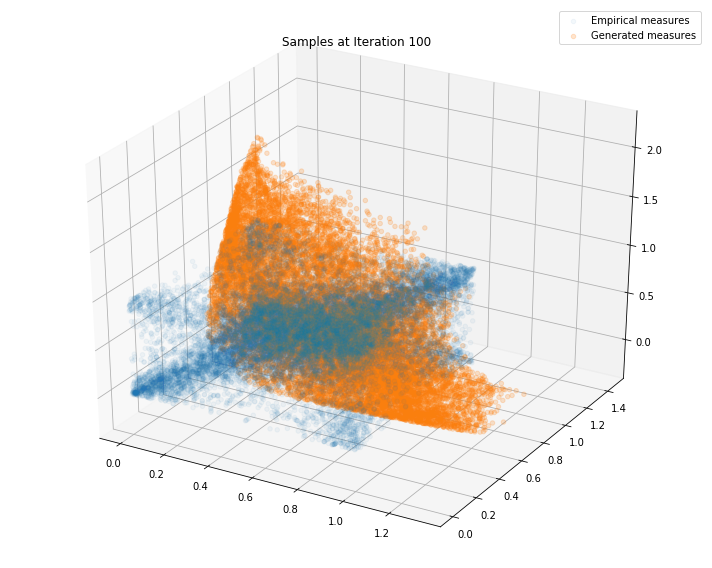
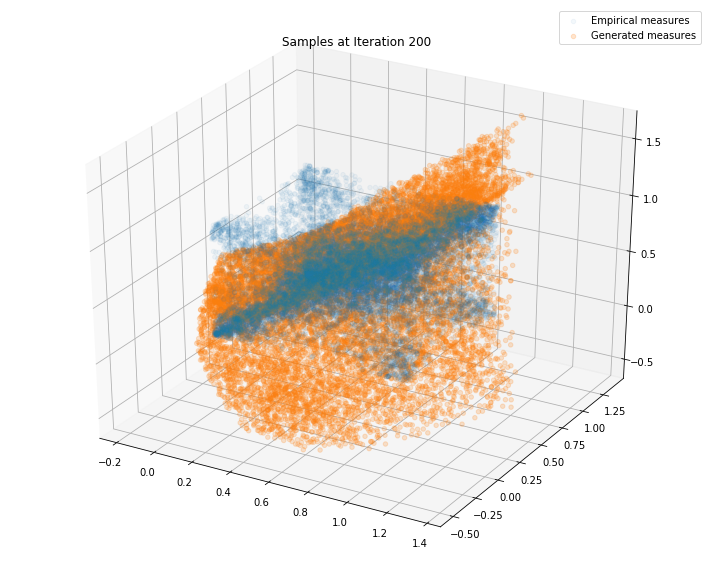
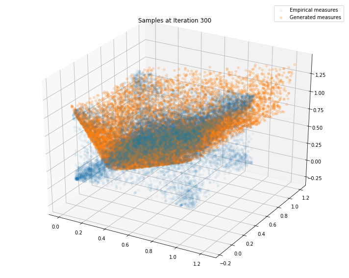
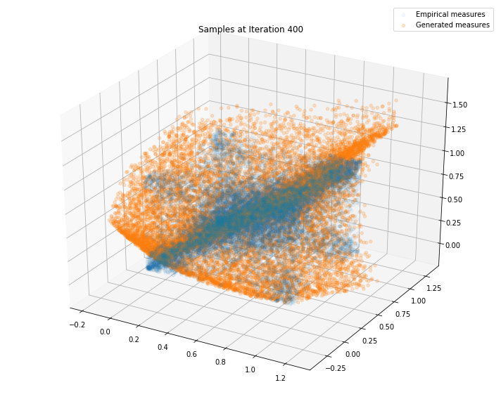
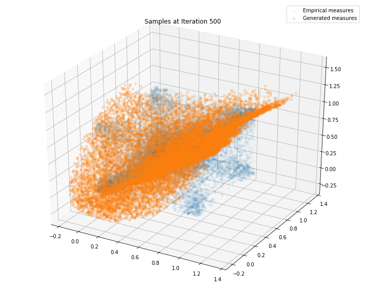
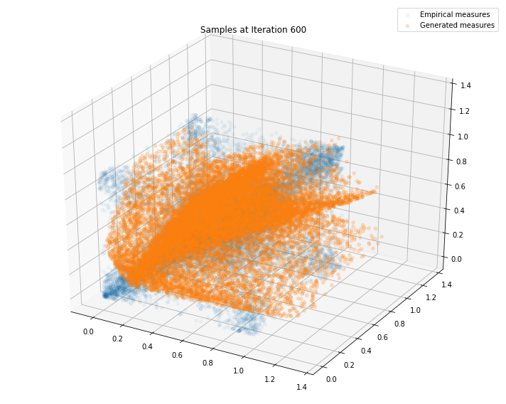
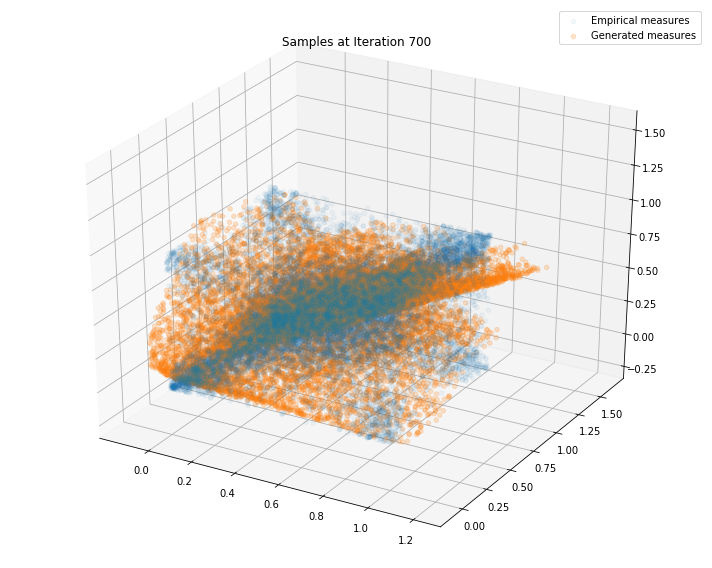
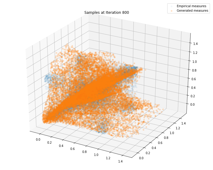
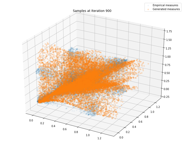
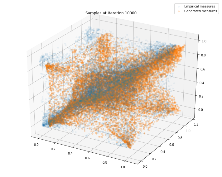
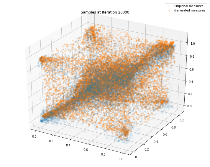
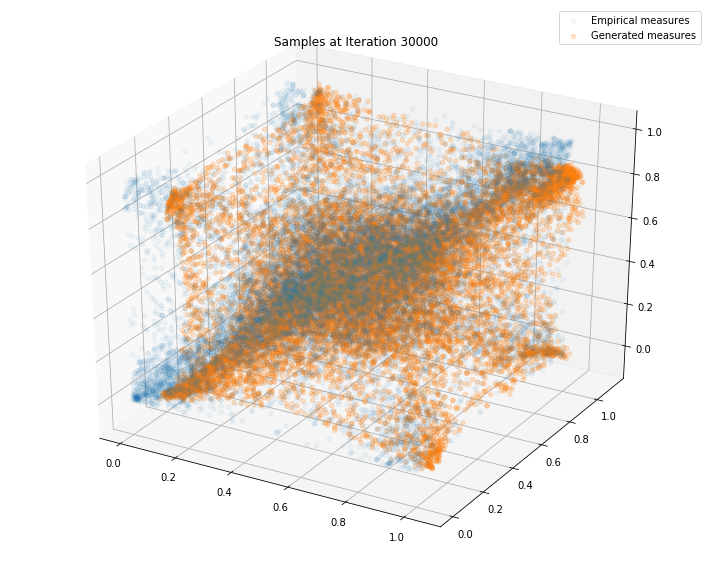
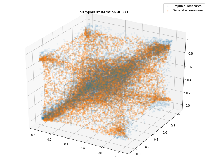
Regularly, we display the GAN distribution (in orange), and the real empirical one (in blue). We can see how the orange starts to progressively match the blue one.
We also display 3 faces, and for each face 3 heatmaps:
- (leftmost) real empirical 2d distribution (after projection on that face),
- (center) GAN generated 2d distribution (after projection on that face),
- (rightmost) 2d distribution of the ranked GAN generated points.
for i in range(50000 + 1):
    X_batch = sample_from_copula(n=batch_size)
    Z_batch = sample_Z(batch_size, 3)

    for _ in range(nd_steps):
        _, dloss = sess.run([disc_step, disc_loss],
                            feed_dict={X: X_batch, Z: Z_batch})
    rrep_dstep, grep_dstep = sess.run([r_rep, g_rep],
                                      feed_dict={X: X_batch, Z: Z_batch})

    for _ in range(ng_steps):
        _, gloss = sess.run([gen_step, gen_loss],
                            feed_dict={Z: Z_batch})

    rrep_gstep, grep_gstep = sess.run([r_rep, g_rep],
                                      feed_dict={X: X_batch, Z: Z_batch})

    # analytics display
    if (i <= 1000 and i % 100 == 0) or (i % 10000 == 0):
        print("Iterations: %d\t Discriminator loss: %.4f\t Generator loss: %.4f"
            % (i, dloss, gloss))

        fig = plt.figure(figsize=(10, 8))
        g_plot = sess.run(G_sample, feed_dict={Z: Z_plot})
        ax = fig.add_subplot(111, projection='3d')
        ax.scatter(x_plot[:, 0], x_plot[:, 1], x_plot[:, 2], alpha=0.05)
        ax.scatter(g_plot[:, 0], g_plot[:, 1], g_plot[:, 2], alpha=0.2)

        plt.legend(["Empirical measures", "Generated measures"])
        plt.title('Samples at Iteration %d' % i)
        plt.tight_layout()
        plt.show()
        plt.close()

        plot_faces(x_plot, g_plot)
Iterations: 0 Discriminator loss: 1.3303 Generator loss: 0.6944
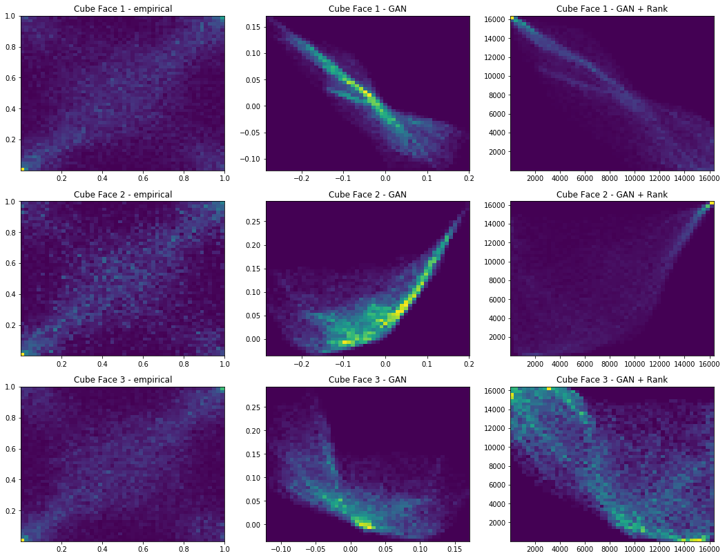
Iterations: 100 Discriminator loss: 1.3862 Generator loss: 0.7905
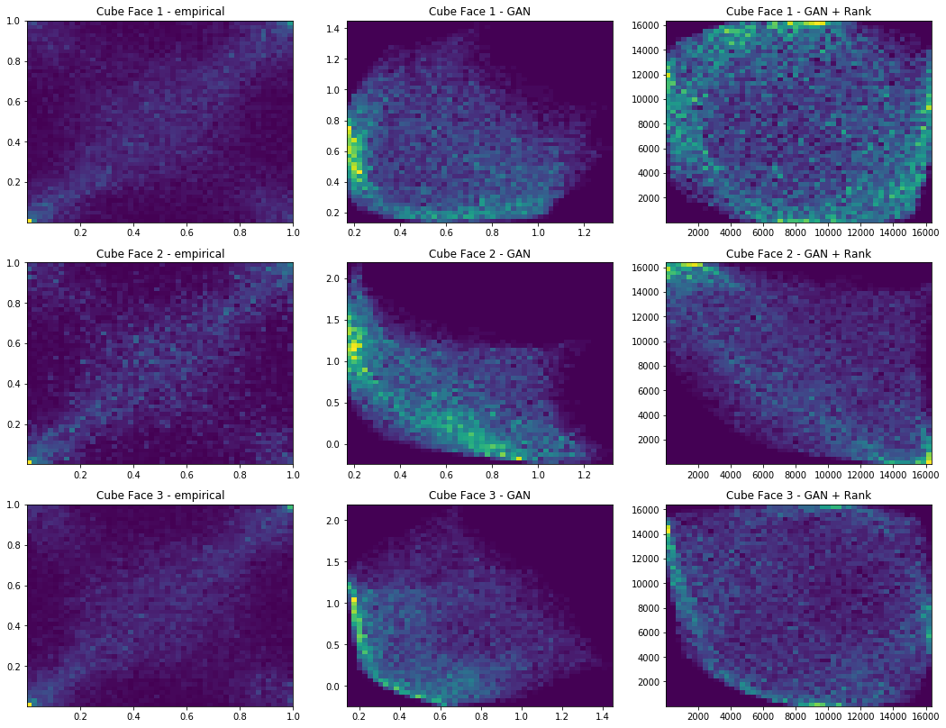
Iterations: 200 Discriminator loss: 1.3827 Generator loss: 0.6865
Iterations: 300 Discriminator loss: 1.3778 Generator loss: 0.7033
Iterations: 400 Discriminator loss: 1.3750 Generator loss: 0.6767
Iterations: 500 Discriminator loss: 1.3625 Generator loss: 0.6953
Iterations: 600 Discriminator loss: 1.3821 Generator loss: 0.7045
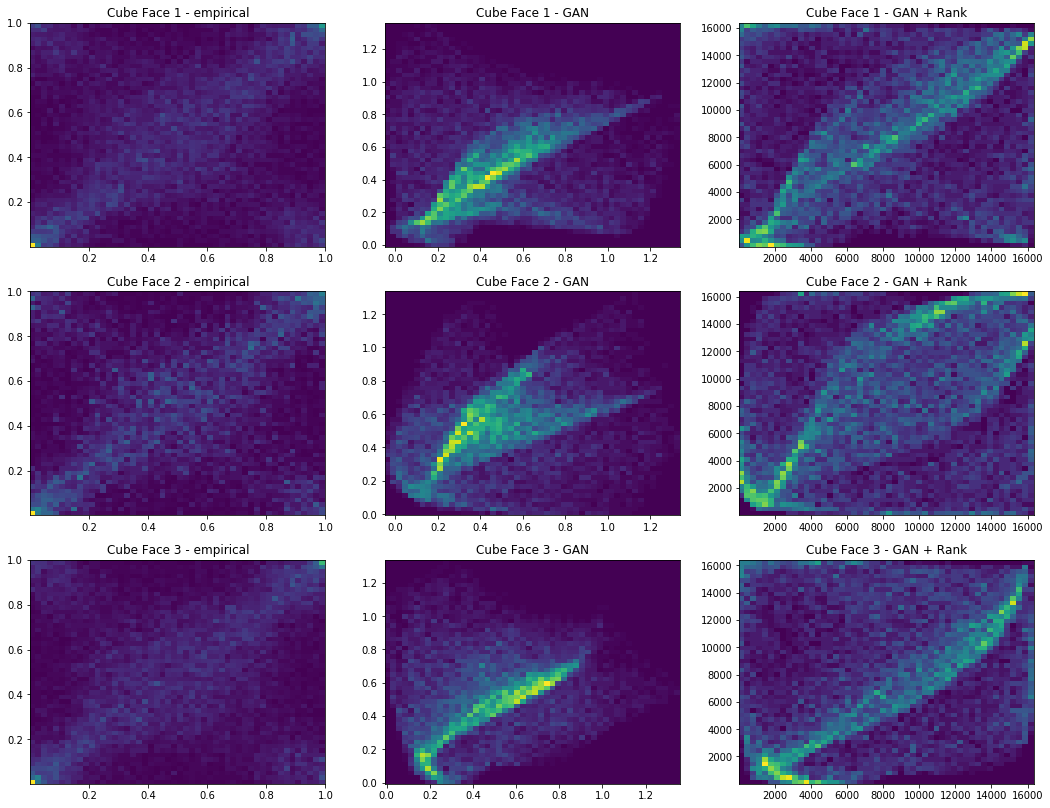
Iterations: 700 Discriminator loss: 1.3709 Generator loss: 0.7060
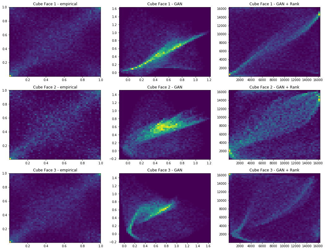
Iterations: 800 Discriminator loss: 1.3778 Generator loss: 0.7035
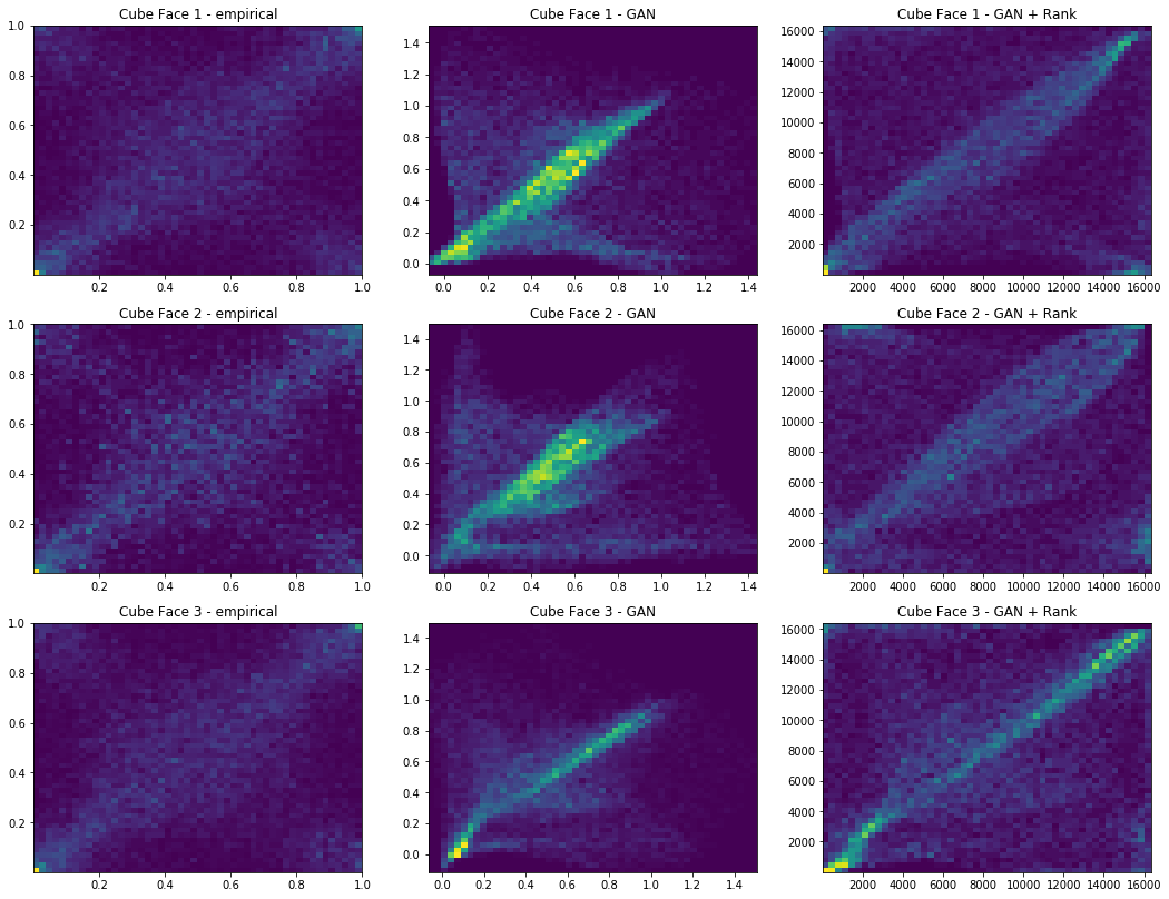
Iterations: 900 Discriminator loss: 1.3773 Generator loss: 0.7076
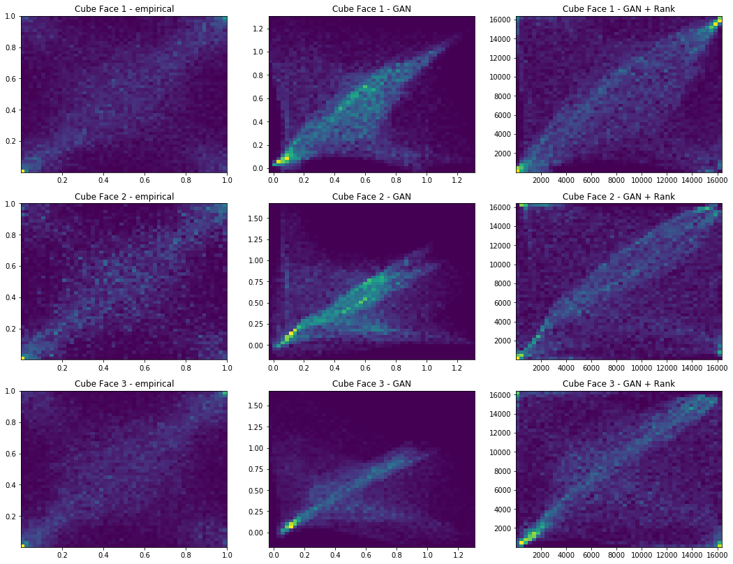
Iterations: 1000 Discriminator loss: 1.3819 Generator loss: 0.6921
Iterations: 10000 Discriminator loss: 1.3823 Generator loss: 0.6756
Iterations: 20000 Discriminator loss: 1.3836 Generator loss: 0.7046
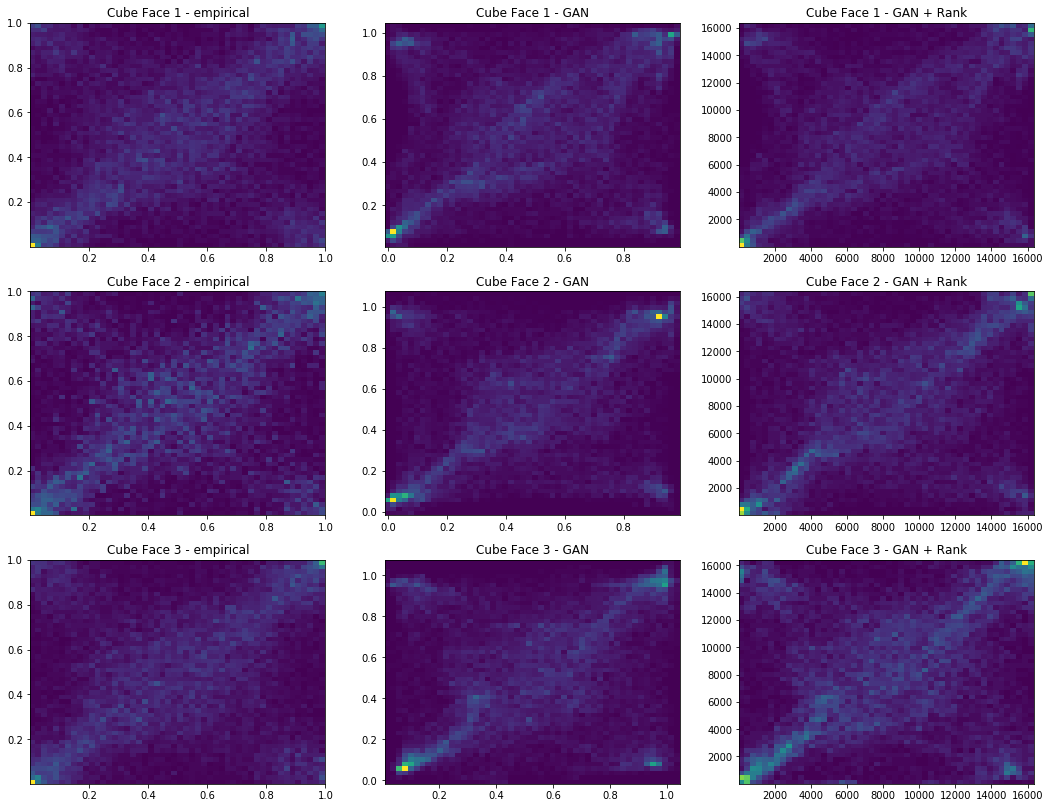
Iterations: 30000 Discriminator loss: 1.3753 Generator loss: 0.7269
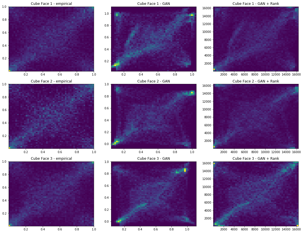
Iterations: 40000 Discriminator loss: 1.3840 Generator loss: 0.7027
Iterations: 50000 Discriminator loss: 1.3743 Generator loss: 0.7234
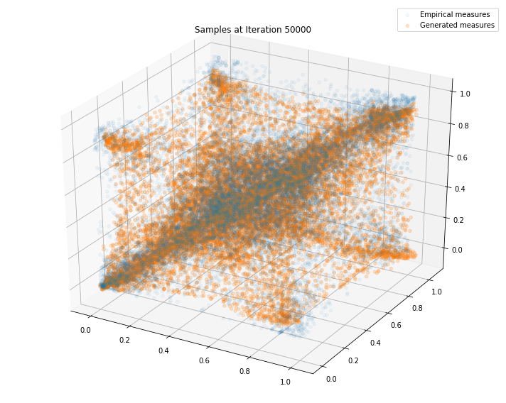
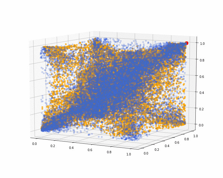
We can see that this basic GAN has managed to roughly match the original distribution.
We show the 3d point cloud (after ranking and normalizing into $[0, 1]^3$) produced by the last iteration of the GAN training (in orange; original distribution in blue; red dot as visual clue for (1, 1, 1)):
xs = x_plot[:, 0]
ys = x_plot[:, 1]
zs = x_plot[:, 2]

xgan = g_plot[:, 0]
ygan = g_plot[:, 1]
zgan = g_plot[:, 2]

xrgan = rankdata(xgan) / len(xgan)
yrgan = rankdata(ygan) / len(ygan)
zrgan = rankdata(zgan) / len(zgan)

fig = plt.figure(figsize=(10, 8))
ax = plt.axes(projection='3d')
ax.scatter(xs, ys, zs,
           color='royalblue', alpha=0.05)
ax.scatter(xrgan, yrgan, zrgan,
           color='orange', alpha=0.2)
ax.scatter(1, 1, 1, color='red', s=100)
ax.view_init(30, 45)
plt.tight_layout()
plt.show()
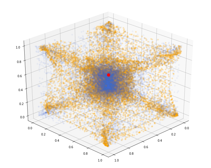
We can see that some corners are missing. I have been able to obtain (visually) better results on different runs, but it is rather difficult to decide when to stop training on an objective criterion.
def init():
    ax.scatter(xs, ys, zs,
               color='royalblue', alpha=0.05)
    ax.scatter(xrgan, yrgan, zrgan,
               color='orange', alpha=0.2)
    ax.scatter(1, 1, 1, color='red', s=100)
    return fig,

def animate_mpg(i):
    if i < 90:
        ax.view_init(elev=10, azim=i*4)
    elif i < 180:
        ax.view_init(elev=10+2*(i%90), azim=(i%90)*4)
    else:
        ax.view_init(elev=190-2*(i%90), azim=0)
    return fig,

def animate_gif(i):
    if i < 90:
        ax.view_init(elev=10, azim=-60+i*4)
    elif i < 133:
        ax.view_init(elev=10+(i%90)*4, azim=-60)
    else:
        ax.view_init(elev=-180+(10+(i%90)*4)%180, azim=-60)
    return fig,
And, to conclude, the associated animation:
fn = 'figs/gan_copula_3d'

anim = animation.FuncAnimation(
    fig, animate_mpg, init_func=init, frames=270, interval=50,
    blit=True)

anim.save(fn + '.mp4', writer='ffmpeg', fps=1000 / 50)

anim = animation.FuncAnimation(
    fig, animate_gif, init_func=init, frames=180, interval=50,
    blit=True)

anim.save(fn + '.gif', writer='imagemagick', fps=1000 / 50)
Conclusion: Results are encouraging to extend to higher dimensions. One promising research avenue is to try Stochastic Deep Networks for this problem. We also need to develop a better understanding of the characteristics of these empirical distributions (aka stylized facts), which can both help design a suitable network and check whether its results are relevant.