Permutation invariance in Neural networks
Permutation invariance in Neural networks
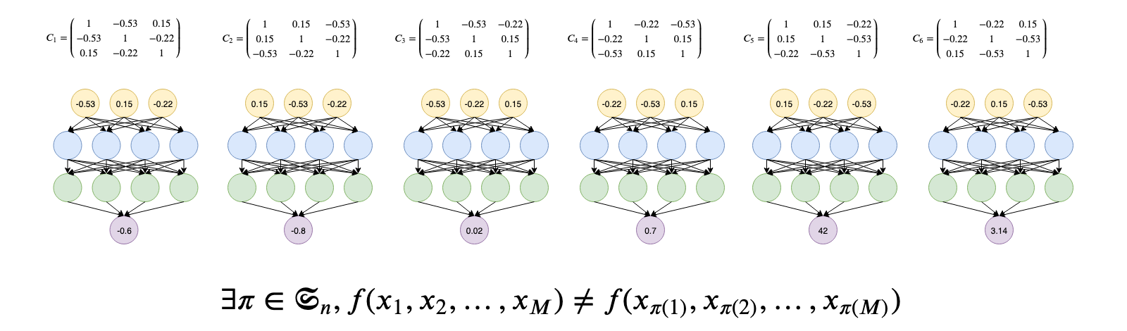 Standard neural networks are not permutation invariant. That is changing the order of their inputs may yield to different outputs as illustrated above. For some tasks, this is an unwanted behaviour.
In this blog, we highlight the limitations of a naive approach which puts too much faith in standard neural network architectures to solve any problems.
I illustrate the point on a concrete example: A regression and a classification tasks whose inputs are the coefficients of a correlation matrix.
This example comes from my recent attempts at developping a Generative Adversarial Network (GAN) to sample realistic financial correlation matrices (blog 1, blog 2, blog 3): I need a discriminator network which can be able to classify whether a given correlation matrix is realistic or not.
Regression task [illustrated at the top]:
Given a set of coefficients (the upper diagonal of a correlation matrix), output the sum of its values.
Classification task:
Consider a finite number of equivalence classes for the relation “there exists a permutation of the rows and columns of the matrix such that they are equal” which are indexed by an integer.
Given a matrix (known to be a member of one of the equivalence classes), output the index (an integer) of the class.
TL;DR When permutation invariance matters, standard neural networks can underperform by orders of magnitude special architectures designed to deal with permutation invariance. One explanation is that the standard neural networks are not data efficient: For 1 point (input) of dimension n, there exist n! equivalent points (inputs). Since the factorial function grows amazingly fast, it prevents a brute force approach, i.e. labeling and training on many if not all the equivalent points, for example 10! = 3,628,800; 20! = 2,432,902,008,176,640,000; 100! ~= 9.3 × 10^157.
Now, let’s illustrate all that with some code:
First, some imports.
%matplotlib inline

import os
os.environ["CUDA_VISIBLE_DEVICES"] = '0'
import itertools
from collections import namedtuple

import matplotlib.pyplot as plt
import numpy as np
import pandas as pd
import tensorflow as tf
import keras
from keras.models import (
    Sequential, Model, load_model)
from keras.layers import (
    Activation, Dense, Dropout,
    Input, Embedding, Lambda)
from keras.optimizers import Adam
from keras.callbacks import ModelCheckpoint
from keras.utils import to_categorical
from keras.objectives import MSE, MAE
from keras.callbacks import EarlyStopping
from tqdm import tqdm, trange
from sklearn.model_selection import train_test_split
from sklearn.metrics import (
    mean_absolute_error, mean_squared_error,
    median_absolute_error, r2_score,
    accuracy_score)
The following snippet is useful for sampling random correlation matrices according to a uniform distribution on their support the elliptope (cf. this blog for details).
from numpy.random import beta
from numpy.random import randn
from scipy.linalg import sqrtm
from numpy.random import seed


def sample_unif_correlmat(dimension):
    d = dimension + 1

    prev_corr = np.matrix(np.ones(1))
    for k in range(2, d):
        # sample y = r^2 from a beta distribution
        # with alpha_1 = (k-1)/2 and alpha_2 = (d-k)/2
        y = beta((k - 1) / 2, (d - k) / 2)
        r = np.sqrt(y)

        # sample a unit vector theta uniformly
        # from the unit ball surface B^(k-1)
        v = randn(k-1)
        theta = v / np.linalg.norm(v)

        # set w = r theta
        w = np.dot(r, theta)

        # set q = prev_corr**(1/2) w
        q = np.dot(sqrtm(prev_corr), w)

        next_corr = np.zeros((k, k))
        next_corr[:(k-1), :(k-1)] = prev_corr
        next_corr[k-1, k-1] = 1
        next_corr[k-1, :(k-1)] = q
        next_corr[:(k-1), k-1] = q

        prev_corr = next_corr

    return next_corr
The following two functions are used to permute rows and columns of a given correlation matrix.
The first function generates several equivalent correlation matrices from a given one by applying the list of permutations given in parameter.
The second one returns a correlation matrix which can be considered as the representative of the equivalence class. The trick to find this representative is to use the permutation defined by sorting the rows (or columns) according to the sum of their coefficients (probability of ties being negligible).
def generate_corr_permutations(corr, permutations):
    X = []
    for permutation in permutations:
        prows = corr[permutation, :]
        perm = prows[:, permutation]
        X.append(perm)

    return X

def canonical_repr(corr):
    permutation = corr.sum(axis=1).argsort()
    prows = corr[permutation, :]
    perm = prows[:, permutation]

    return perm
Let’s see how it works through a simple example.
Let’s consider for now 3x3 correlation matrices. We sample one randomly. We generate all the possible permutations: 3! = 1 * 2 * 3 = 6.
dim = 3
permutations = list(itertools.permutations(range(dim)))

corr = sample_unif_correlmat(dim)
perm_corr = generate_corr_permutations(corr, permutations)
Here are all the equivalent matrices (also displayed in the illustration at the top):
for corr in perm_corr:
    print(corr)
[[ 1.         -0.53190206  0.15400023]
 [-0.53190206  1.         -0.21892359]
 [ 0.15400023 -0.21892359  1.        ]]
[[ 1.          0.15400023 -0.53190206]
 [ 0.15400023  1.         -0.21892359]
 [-0.53190206 -0.21892359  1.        ]]
[[ 1.         -0.53190206 -0.21892359]
 [-0.53190206  1.          0.15400023]
 [-0.21892359  0.15400023  1.        ]]
[[ 1.         -0.21892359 -0.53190206]
 [-0.21892359  1.          0.15400023]
 [-0.53190206  0.15400023  1.        ]]
[[ 1.          0.15400023 -0.21892359]
 [ 0.15400023  1.         -0.53190206]
 [-0.21892359 -0.53190206  1.        ]]
[[ 1.         -0.21892359  0.15400023]
 [-0.21892359  1.         -0.53190206]
 [ 0.15400023 -0.53190206  1.        ]]
And now, we verify that each of these 6 matrices are mapped to the same representative:
for corr in perm_corr:
    print(canonical_repr(corr))
[[ 1.         -0.53190206 -0.21892359]
 [-0.53190206  1.          0.15400023]
 [-0.21892359  0.15400023  1.        ]]
[[ 1.         -0.53190206 -0.21892359]
 [-0.53190206  1.          0.15400023]
 [-0.21892359  0.15400023  1.        ]]
[[ 1.         -0.53190206 -0.21892359]
 [-0.53190206  1.          0.15400023]
 [-0.21892359  0.15400023  1.        ]]
[[ 1.         -0.53190206 -0.21892359]
 [-0.53190206  1.          0.15400023]
 [-0.21892359  0.15400023  1.        ]]
[[ 1.         -0.53190206 -0.21892359]
 [-0.53190206  1.          0.15400023]
 [-0.21892359  0.15400023  1.        ]]
[[ 1.         -0.53190206 -0.21892359]
 [-0.53190206  1.          0.15400023]
 [-0.21892359  0.15400023  1.        ]]
Works.
Enough introduction. Now we can benchmark the performance of a vanilla Multi-Layer Perceptron (MLP) vs. the same model which is permutation invariant. To make it simple, we enforce the permutation invariance using the representative trick. You can also play with Deep Sets and the variants for enforcing the permutation invariance in the neural network itself.
Digression: Using a “Deep Sets” model, results where in between the vanilla MLP (worst results) and the pure permutation invariant approach using the representative (best results): Most of the time, for small dimensions, “Deep Sets” was slightly underperforming the best model yet some unstability could make it worse than the vanilla MLP from time to time; for higher dimensions, I got relatively weak results with the “Deep Sets” overperforming slightly the vanilla MLP.
Let’s define the following function to generate training, validation, and testing data:
def generate_data(dim, nb_classes=10, nb_examples=1000, use_canon_repr=False):
    permutations = [np.random.permutation(range(dim))
                    for i in range(nb_examples)]

    X = []
    y_sum = []
    y_class = []

    for id_class in range(nb_classes):
        corr = sample_unif_correlmat(dim)
        perm_corrs = generate_corr_permutations(corr, permutations)

        for perm_corr in perm_corrs:
            if use_canon_repr:
                perm_corr = canonical_repr(perm_corr)
            a, b = np.triu_indices(dim, k=1)
            vec_corr = perm_corr[a, b]

            X.append(vec_corr)
            y_sum.append(round(vec_corr.sum(), 4))
            y_class.append(id_class)

    X = np.array(X)
    y_sum = np.array(y_sum)
    y_class = np.array(y_class)

    permutation = np.random.permutation(len(X))

    X = X[permutation, :]
    y_sum = y_sum[permutation]
    y_class = y_class[permutation]

    return X, y_sum, y_class
Basically, this function takes as input the size of the matrix (dim x dim), the number of equivalence classes, the number of samples per class, and whether to map the samples to their class representative. For each class, we sample randomly a correlation matrix, and then we generate nb_examples equivalent ones by permutations. Finally, for each of the (nb_classes * nb_examples) samples, we extract the upper diagonal of dim * (dim - 1) / 2 coefficients, and flatten it to a vector corresponding to one row in the data X of shape (nb_classes * nb_examples, dim * (dim - 1) / 2).
We define two target variables:
- y_sum, for the regression task, a vector of size (nb_classes * nb_examples) which contains the sum of the dim * (dim - 1) / 2 coefficients of each sample;
- y_class, for the classification task, a vector of size (nb_classes * nb_examples) which contains the index of the equivalence class of each sample.
That’s it.
N.B. The final permutation on X, y_sum, y_class is unrelated to the data generation, and not strictly necessary: Shuffling the rows in X, y just to make sure to have some diversity in the learning batches (usually taken care of automatically by modern ml libraries).
Regression task [illustrated at the top]:
Given a set of coefficients (the upper diagonal of a correlation matrix), output the sum of its values.
We define 10 classes, that is essentially 10 different correlation matrices (and thus, with high probability 10 different sums). For each of these 10 classes, we generate 600 samples: essentially, permutations of the representative of the class. In cases where dimensionality is small (say 3) many samples are therefore identical (as there are only 3! = 6 possible matrices in this case). But rapidly dimensionality becomes too big so that the 600 samples are enough to cover a significant proportion of all the possible permutations (6! = 720 > 600). Thus, there will be matrices in the test set unseen during the training.
Can a vanilla architecture (such as the MLP) generalize well enough?
Code for training and evaluating the MLP on this regression task:
vector_sizes = []
mae = []

nb_classes = 10
nb_examples = 600

for dim in range(3, 101):

    X, y_sum, y_class = generate_data(
        dim, nb_classes=nb_classes, nb_examples=nb_examples,
        use_canon_repr=False)

    X_train, X_test, y_train, y_test = train_test_split(
        X, y_sum, test_size=0.2, random_state=42)

    model = Sequential()
    model.add(Dense(input_dim=X_train.shape[1], units=256))
    model.add(Activation("tanh"))
    model.add(Dropout(rate=0.50))
    model.add(Dense(units=128))
    model.add(Activation("relu"))
    model.add(Dropout(rate=0.50))
    model.add(Dense(units=64))
    model.add(Activation("relu"))
    model.add(Dropout(rate=0.50))
    model.add(Dense(units=1))
    model.compile("nadam", "mae")

    early_stopping = EarlyStopping(monitor='val_loss', patience=50)
    checkpointer = ModelCheckpoint(filepath='/tmp/weights.hdf5',
                                   verbose=0, save_best_only=True)

    model.fit(X_train, y_train,
              batch_size=256, epochs=200,
              validation_split=0.2, verbose=0,
              callbacks=[checkpointer, early_stopping])

    model = load_model('/tmp/weights.hdf5')

    vector_sizes.append(X_train.shape[1])
    mae.append(mean_absolute_error(
        y_test, model.predict(X_test)))

vanilla_mae = pd.Series(mae, index=vector_sizes)
As a baseline, code for training and evaluating the same MLP but using as input a permutation invariant representation:
vector_sizes = []
mae = []

nb_classes = 10
nb_examples = 600

for dim in range(3, 101):

    X, y_sum, y_class = generate_data(
        dim, nb_classes=nb_classes, nb_examples=nb_examples,
        use_canon_repr=True)

    X_train, X_test, y_train, y_test = train_test_split(
        X, y_sum, test_size=0.2, random_state=42)

    model = Sequential()
    model.add(Dense(input_dim=X_train.shape[1], units=256))
    model.add(Activation("tanh"))
    model.add(Dropout(rate=0.50))
    model.add(Dense(units=128))
    model.add(Activation("relu"))
    model.add(Dropout(rate=0.50))
    model.add(Dense(units=64))
    model.add(Activation("relu"))
    model.add(Dropout(rate=0.50))
    model.add(Dense(units=1))
    model.compile("nadam", "mae")

    early_stopping = EarlyStopping(monitor='val_loss', patience=50)
    checkpointer = ModelCheckpoint(filepath='/tmp/weights.hdf5',
                                   verbose=0, save_best_only=True)

    model.fit(X_train, y_train,
              batch_size=256, epochs=200,
              validation_split=0.2, verbose=0,
              callbacks=[checkpointer, early_stopping])

    model = load_model('/tmp/weights.hdf5')

    vector_sizes.append(X_train.shape[1])
    mae.append(mean_absolute_error(
        y_test, model.predict(X_test)))

sorted_vanilla_mae = pd.Series(mae, index=vector_sizes)
We display the evolution of the mean absolute error as a function of the growing dimension (more possible permutations for a fixed number of samples):
plt.figure(figsize=(12, 9))
plt.plot(vanilla_mae, label='vanilla nn')
plt.plot(sorted_vanilla_mae, label='vanilla nn w/ invariance')
plt.xlabel('dim * (dim - 1) / 2', fontsize=16)
plt.ylabel('MAE', fontsize=16)
plt.legend(fontsize=16)
plt.title("Mean absolute error as a function of the input " +
          "vector size = dim * (dim - 1) / 2",
          fontsize=16)
plt.show()
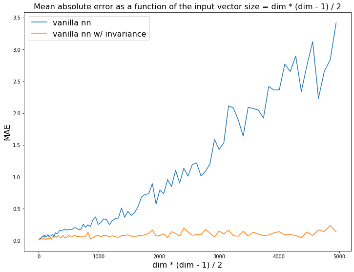 Regression task: Estimate the sum of the dim * (dim - 1) / 2 coefficients from the upper diagonal of the correlation matrix. The vanilla MLP is not data efficient enough and struggles to generalize to permutations of the input it has never seen.
Conclusion: The vanilla MLP is not data efficient. The naive approach would require far too much data to be able to work. Encoding invariance relevant to the problem at hand in the model definitely helps! Sometimes, invariance can be “manually” encoded in the input (like here), or in the neural network architecture (like in Deep Sets for permutation invariance, or typically a standard Convolutional Neural Network (CNN) for translation invariance).