Stylized Facts of Financial Correlations
Stylized Facts of Financial Correlations
In a previous blog CorrGAN: A GAN for sampling correlation matrices (Part II), we have shown how to devise a GAN to sample realistic 3x3 financial correlation matrices. Not too hard, and not too useful either. Before going further, and being able to generate realistic nxn correlation matrices for any n (say, n less than 10,000), we need to solve a few problems we didn’t encounter for the 3x3 case.
-
How to be sure we sample from the whole sub-space of realistic financial correlation matrices (and not just memorizing a tiny subset of it… which would defeat the whole purpose of using a GAN in the first place)?
-
How to be sure that the correlation matrices sampled from the GAN are indeed realistic (i.e. they share the same statistical features than the ones estimated from real financial returns)?
In this blog post, we tackle 2.
Some stylized facts are known in the stat quant literature:
1. Distribution of pairwise correlations is significantly shifted to the positive,
2. Eigenvalues follow the Marchenko–Pastur distribution, but for
    a. a very large first eigenvalue,
    b. a couple of other large eigenvalues,
3. Perron-Frobenius property (first eigenvector has positive entries),
4. Hierarchical structure of clusters,
5. Scale-free property of the corresponding MST.
Below some code that helps checking these properties.
import pandas as pd
import numpy as np
from numpy.random import beta
from numpy.random import randn
from scipy.linalg import sqrtm
from numpy.random import seed
from random import randint
import networkx as nx
import matplotlib.pyplot as plt
import seaborn as sns

%matplotlib inline
nb_assets = 100
corrs = pd.read_hdf('./corrs/sample_{}x{}_correls.h5'.format(nb_assets, nb_assets))
sample_size = corrs.shape[0]
corrs.shape
(951, 4950)
corrs_sq = []
for mat in corrs.values:
    corr = np.eye(nb_assets)
    corr[np.triu_indices(nb_assets, k=1)] = mat
    i_lower = np.tril_indices(nb_assets, -1)
    corr[i_lower] = corr.T[i_lower]
    corrs_sq.append(corr)

len(corrs_sq), corrs_sq[0].shape
(951, (100, 100))
Sample uniformly random correlation matrices from the whole 4950-dimensional elliptope
def sample_unif_correlmat(dimension):
    d = dimension + 1

    prev_corr = np.matrix(np.ones(1))
    for k in range(2, d):
        # sample y = r^2 from a beta distribution with alpha_1 = (k-1)/2 and alpha_2 = (d-k)/2
        y = beta((k - 1) / 2, (d - k) / 2)
        r = np.sqrt(y)

        # sample a unit vector theta uniformly from the unit ball surface B^(k-1)
        v = randn(k-1)
        theta = v / np.linalg.norm(v)

        # set w = r theta
        w = np.dot(r, theta)

        # set q = prev_corr**(1/2) w
        q = np.dot(sqrtm(prev_corr), w)

        next_corr = np.zeros((k, k))
        next_corr[:(k-1), :(k-1)] = prev_corr
        next_corr[k-1, k-1] = 1
        next_corr[k-1, :(k-1)] = q
        next_corr[:(k-1), k-1] = q

        prev_corr = next_corr

    return next_corr

def vectorize(mats):
    return np.array(
        [list(m[np.triu_indices(nb_assets, k=1)]) for m in mats])

def sample_data(n=10000):
    data = []
    for i in range(n):
        m = sample_unif_correlmat(nb_assets)
        data.append(m)

    return data

uniform_sq = sample_data(sample_size)
uniform = vectorize(uniform_sq)
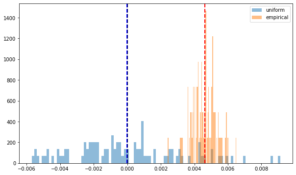
1. Correlation coefficients are mostly positive, and their mean usually above 0.3
all_coeffs = corrs.values.reshape(corrs.values.shape[0] * corrs.values.shape[1])
coeffs_unif = uniform.reshape(uniform.shape[0] * uniform.shape[1])
plt.figure(figsize=(10, 10))
plt.hist(coeffs_unif, bins=200, log=False, density=True, alpha=0.5, label='uniform')
plt.hist(all_coeffs, bins=200, log=False, density=True, alpha=0.5, label='empirical')
plt.axvline(x=np.mean(all_coeffs), color='r', linestyle='dashed', linewidth=2)
plt.axvline(x=np.mean(coeffs_unif), color='b', linestyle='dashed', linewidth=2)
plt.legend()
plt.show()

2. Correlation matrices eigenspectrum follows the Marchenko–Pastur law, with a few large eigenvalues, and one extremely large
The seminal paper Random matrix theory and financial correlations has shown that empirical correlation matrices estimated on returns share statistical features with random matrices: Their respective eigenspectrum largely overlap, but for a few large eigenvalues (corresponding more or less to sectors) and a very large one (corresponding to the ‘market’).
def compute_eigenvals(correls):
    eigenvalues = []
    for corr in correls:
        eigenvals, eigenvecs = np.linalg.eig(corr)
        eigenvalues.append(sorted(eigenvals, reverse=True))

    return eigenvalues

sample_mean_eigenvals = np.mean(compute_eigenvals(corrs_sq), axis=0)
sample_mean_unif_eigenvals = np.mean(compute_eigenvals(uniform_sq), axis=0)
plt.figure(figsize=(10, 6))
plt.hist(sample_mean_unif_eigenvals, bins=nb_assets, density=True, alpha=0.5, label='uniform')
plt.hist(sample_mean_eigenvals, bins=nb_assets, density=True, alpha=0.5, label='empirical')
plt.legend()
plt.show()

3. Correlation matrices verify the Perron–Frobenius theorem
Perron–Frobenius theorem:
In linear algebra, the Perron–Frobenius theorem, proved by Oskar Perron (1907) and Georg Frobenius (1912), asserts that a real square matrix with positive entries has a unique largest real eigenvalue and that the corresponding eigenvector can be chosen to have strictly positive components.
def compute_pf_vec(correls):
    pf_vectors = []
    for corr in correls:
        eigenvals, eigenvecs = np.linalg.eig(corr)
        pf_vectors.append(eigenvecs[:, np.argmax(eigenvals)])

    return pf_vectors

mean_pf = np.mean(compute_pf_vec(corrs_sq), axis=0)
mean_unif_pf = np.mean(compute_pf_vec(uniform_sq), axis=0)
plt.figure(figsize=(10, 6))
plt.hist(mean_unif_pf, bins=nb_assets, density=True, alpha=0.5, label='uniform')
plt.hist(mean_pf, bins=nb_assets, density=True, alpha=0.5, label='empirical')
plt.axvline(x=0, color='k', linestyle='dashed', linewidth=2)
plt.axvline(x=np.mean(mean_pf), color='r', linestyle='dashed', linewidth=2)
plt.axvline(x=np.mean(mean_unif_pf), color='b', linestyle='dashed', linewidth=2)
plt.legend()
plt.show()
4. Correlation matrices have a hierarchical structure
This stylized fact was first noticed by Mantegna in his seminal paper Hierarchical Structure in Financial Markets.
for idx, corr in enumerate(corrs_sq):
    sns.clustermap(corr)

    if idx > 5:
        break


for idx, corr in enumerate(uniform_sq):
    sns.clustermap(corr)

    if idx > 5:
        break


5. Minimum Spanning Trees extracted from correlation matrices have node degrees seemingly following a power law
Non-random topology of stock markets has been one of the first paper to document that the degree of a node in the MST extracted from financial correlations follows (seemingly) a power law, but for a few nodes with high degrees (cf. Figure 5. in Emergence of Complexity in Financial Networks).
def compute_degree_counts(correls):
    all_counts = []
    for corr in correls:
        dist = (1 - corr) / 2
        G = nx.from_numpy_matrix(dist)
        mst = nx.minimum_spanning_tree(G)

        degrees = {i: 0 for i in range(nb_assets)}
        for edge in mst.edges:
            degrees[edge[0]] += 1
            degrees[edge[1]] += 1
        degrees = pd.Series(degrees).sort_values(ascending=False)
        cur_counts = degrees.value_counts()
        counts = np.zeros(nb_assets)
        for i in range(nb_assets):
            if i in cur_counts:
                counts[i] = cur_counts[i]

        all_counts.append(counts / (nb_assets - 1))

    return all_counts
mean_counts = np.mean(compute_degree_counts(corrs_sq), axis=0)
mean_counts = pd.Series(mean_counts).replace(0, np.nan)

mean_unif_counts = np.mean(compute_degree_counts(uniform_sq), axis=0)
mean_unif_counts = pd.Series(mean_unif_counts).replace(0, np.nan)
plt.figure(figsize=(10, 6))
plt.scatter(mean_unif_counts.index, mean_unif_counts, label='uniform')
plt.scatter(mean_counts.index, mean_counts, label='empirical')
plt.legend()
plt.show()

plt.figure(figsize=(10, 6))
plt.scatter(np.log10(mean_unif_counts.index), np.log10(mean_unif_counts), label='uniform')
plt.scatter(np.log10(mean_counts.index), np.log10(mean_counts), label='empirical')
plt.legend()
plt.show()

Conclusion: These “stylized facts” seem quite robust and specific to financial correlations: They can be useful to verify that correlation matrices generated by GANs are realistic.