Building a S&P 500 company classification from Wikipedia articles (guided by ChatGPT)
Building a S&P 500 company classification from Wikipedia articles (guided by ChatGPT)
Collaboration with ChatGPT. I am still useful to package the experiment, and advertise it, but for how long? :-)
In this joint work, I felt more like the robot copy-pasting rather than the author of the experiment.
Sure, I did the prompting, but that too could be automated, after all building networks out of similarity matrices is well documented… for example, in my review (which is now trivialized by Large Language Models (LLMs), except for the opinionated part).
Is using Wikipedia articles and Sentence Transformers original enough so that it deserves human “creativity”? Maybe, probably not.
I did similar things in the past (say around 2013-2017) using Wikipedia - and BoW, Word2Vec, Doc2Vec instead of Sentence Transformers -, but the time and effort required at the time were a good 100x factor. Now, it can take 10 minutes.
Link to the Google Colab notebook: wikipedia_companies_sentence_transformers.ipynb
Let’s now go through the experiment:
Gautier’s Prompt:
There is a table in Wikipedia containing all the companies in the S&P in the article https://en.wikipedia.org/wiki/List_of_S%26P_500_companies how can I pull all the article titles from this page/table in Python?
ChatGPT’s Answer:
To scrape the Wikipedia page for S&P 500 companies and get the article titles for all the companies, you can use the requests and BeautifulSoup libraries. First, install them using pip:
pip install requests beautifulsoup4Then, use the following code to fetch the Wikipedia page, parse the table, and extract the article titles for all the companies:
import requests
from bs4 import BeautifulSoup

def get_sp500_company_links(wikipedia_url):
    response = requests.get(wikipedia_url)
    soup = BeautifulSoup(response.content, 'html.parser')

    table = soup.find('table', {'class': 'wikitable sortable'})
    rows = table.findAll('tr')

    links = []

    for row in rows[1:]:
        link = row.find('td').find_next('td').find('a')['href']
        links.append(link)

    return links

# Example usage
wikipedia_url = 'https://en.wikipedia.org/wiki/List_of_S%26P_500_companies'
sp500_company_links = get_sp500_company_links(wikipedia_url)

for link in sp500_company_links:
    print(f"https://en.wikipedia.org{link}")
This code fetches the Wikipedia page, finds the table with class wikitable sortable, iterates through the rows, and extracts the article links for each company in the table. The resulting sp500_company_links list contains the relative links to the Wikipedia articles, which can be combined with the base URL (https://en.wikipedia.org) to form the full URLs.
Gautier’s Prompt:
Can you write the Python code that takes as input the text (of a Wikipedia article but it does not matter), split it in sentences or paragraphs that can be fed to a sentence transformer, and then yield one relevant embedding for the whole Wikipedia article.
My goal is to loop over all the wikipedia articles, and obtain one embedding per article.
ChatGPT’s Answer:
To achieve this, you can use the nltk library for sentence tokenization and the sentence-transformers library to get embeddings. First, install the necessary libraries:
pip install nltk sentence-transformersThen, use the following Python code to obtain an embedding for the whole Wikipedia article text:
import numpy as np
import nltk
from sentence_transformers import SentenceTransformer

nltk.download('punkt')

def get_article_embedding(text, model_name='paraphrase-distilroberta-base-v1'):
    # Initialize the SentenceTransformer model
    model = SentenceTransformer(model_name)

    # Tokenize the text into sentences
    sentences = nltk.sent_tokenize(text)

    # Get embeddings for each sentence
    sentence_embeddings = model.encode(sentences)

    # Compute the average embedding for the whole article
    article_embedding = np.mean(sentence_embeddings, axis=0)

    return article_embedding

# Example usage
text = "Your Wikipedia article text here."
embedding = get_article_embedding(text)

print("Article embedding:", embedding)
This code defines a function get_article_embedding that takes the text of a Wikipedia article, tokenizes it into sentences using NLTK’s sent_tokenize, and then computes embeddings for each sentence using the SentenceTransformer model. The function returns the average embedding of all sentences as the relevant embedding for the entire article. You can loop over all the Wikipedia articles you want to process, fetch the article text, and use the get_article_embedding function to obtain an embedding for each article.
Gautier’s Prompt:
How can I pull the plain text of a Wikipedia page with Python?
ChatGPT’s Answer:
To extract the plain text from a Wikipedia page using Python, you can use the wikipedia-api library. First, you need to install the library using pip:
pip install wikipedia-apiThen, you can use the following code to fetch the plain text from a specific Wikipedia page:
import wikipediaapi

def get_wikipedia_text(page_title, language='en'):
    wiki = wikipediaapi.Wikipedia(language)
    page = wiki.page(page_title)

    if page.exists():
        return page.text
    else:
        return None

# Example usage
page_title = 'Python (programming language)'
text = get_wikipedia_text(page_title)
if text:
    print(text)
else:
    print(f"Page '{page_title}' does not exist.")
Replace ‘Python (programming language)’ with the title of the Wikipedia page you want to fetch. The function get_wikipedia_text returns the plain text content of the specified page. If the page doesn’t exist, it returns None.
Gautier’s Prompt:
This piece of code is very slow, can you rewrite it using multiprocessing?
embeddings = {}
for title, content in tqdm(page_content.items()):
    embedding = get_article_embedding(content)
    embeddings[title] = embedding
ChatGPT’s Answer:
To speed up the process using multiprocessing, you can utilize the concurrent.futures library which provides a high-level interface for asynchronously executing callables. Here’s how you can modify the code to process the article embeddings in parallel:
import concurrent.futures
from tqdm import tqdm

def get_embedding_for_title(title_content_pair):
    title, content = title_content_pair
    embedding = get_article_embedding(content)
    return title, embedding

# Example usage
page_content = {
    "Article_Title_1": "Article content 1",
    "Article_Title_2": "Article content 2",
    # ...
}

embeddings = {}

# Define the number of worker processes you want to use
num_workers = 4

with concurrent.futures.ProcessPoolExecutor(max_workers=num_workers) as executor:
    for title, embedding in tqdm(
        executor.map(get_embedding_for_title, page_content.items()), total=len(page_content)
    ):
        embeddings[title] = embedding

print("Embeddings:", embeddings)
This code defines a get_embedding_for_title function that takes a (title, content) tuple and returns the (title, embedding) pair. It then uses the ProcessPoolExecutor to create a pool of worker processes to execute the get_embedding_for_title function asynchronously. The executor.map() function is used to apply the function to all the items in the page_content dictionary. Using tqdm with the total parameter set to the length of the page_content dictionary helps show progress as the parallel processing takes place. Adjust the num_workers variable according to your system’s capabilities (usually the number of available CPU cores) for optimal performance.
Gautier’s Prompt:
I have a pandas dataframe with shape 768 x 498 containing the 768 dimensional embeddings for 498 documents. How can I compute in Python the pairwise cosine similarity between all these 498 embeddings fast?
ChatGPT’s Answer:
You can use the sklearn.metrics.pairwise module to efficiently compute pairwise cosine similarity between your document embeddings. Here’s how to do it: First, install scikit-learn if you haven’t already:
pip install scikit-learnThen, use the following Python code to compute the pairwise cosine similarity for your document embeddings:
import pandas as pd
import numpy as np
from sklearn.metrics.pairwise import cosine_similarity

# Assuming 'df' is your DataFrame with 498 document embeddings, each of 768 dimensions
# Create a sample DataFrame for demonstration
data = np.random.rand(498, 768)
df = pd.DataFrame(data)

# Compute pairwise cosine similarity
cosine_sim_matrix = cosine_similarity(df)

print("Cosine similarity matrix shape:", cosine_sim_matrix.shape)
print("Cosine similarity matrix:", cosine_sim_matrix)
This code assumes that your DataFrame with the document embeddings is stored in the variable df. It uses the cosine_similarity() function from scikit-learn to compute the pairwise cosine similarity between all the 498 embeddings. The resulting cosine_sim_matrix is a 498 x 498 matrix containing the cosine similarity values.
Gautier’s Prompt:
Given a full distance matrix, can you give me the Python code to compute and display a beautiful minimum spanning tree?
ChatGPT’s Answer:
To compute and display a beautiful minimum spanning tree from a full distance matrix, you can use the networkx library for graph-related computations and matplotlib for visualization.
First, install the required libraries if you haven’t already:
pip install networkx matplotlib
Then, use the following Python code to compute and display the minimum spanning tree:
import numpy as np
import networkx as nx
import matplotlib.pyplot as plt

# Assuming 'distance_matrix' is a numpy array with your full distance matrix
# Create a random distance matrix for demonstration
distance_matrix = np.random.rand(10, 10)

# Create a graph from the distance matrix
graph = nx.from_numpy_matrix(distance_matrix)

# Compute the minimum spanning tree
mst = nx.minimum_spanning_tree(graph)

# Visualize the minimum spanning tree
pos = nx.spring_layout(mst, seed=42)  # You can experiment with different layout algorithms
nx.draw(mst, pos, with_labels=True, node_color="skyblue", font_size=10, font_weight="bold", node_size=700)
nx.draw_networkx_edge_labels(mst, pos, edge_labels={(u, v): f"{d['weight']:.2f}" for u, v, d in mst.edges(data=True)}, font_size=9)
plt.title("Minimum Spanning Tree")
plt.show()
This code assumes that you have a numpy array named distance_matrix containing your full distance matrix. It creates a graph using the nx.from_numpy_matrix() function, computes the minimum spanning tree using the nx.minimum_spanning_tree() function, and visualizes the resulting tree using matplotlib.
Note that the layout of the nodes can be adjusted using different layout algorithms provided by networkx. In this example, I used the spring_layout algorithm with a fixed seed for consistent results, but you can experiment with other layout algorithms such as circular_layout, kamada_kawai_layout, or random_layout.
Gautier’s Prompt:
How can I display custom node labels on this graph?
ChatGPT’s Answer:
To display custom node labels on the graph, you can modify the nx.draw() function to exclude the node labels and then use the nx.draw_networkx_labels() function with your custom labels.
Here’s the updated code:
import numpy as np
import networkx as nx
import matplotlib.pyplot as plt

# Assuming 'distance_matrix' is a numpy array with your full distance matrix
# Create a random distance matrix for demonstration
distance_matrix = np.random.rand(10, 10)

# Create a graph from the distance matrix
graph = nx.from_numpy_matrix(distance_matrix)

# Compute the minimum spanning tree
mst = nx.minimum_spanning_tree(graph)

# Create custom labels (for demonstration, we use letters as labels)
custom_labels = {i: chr(65 + i) for i in range(distance_matrix.shape[0])}

# Visualize the minimum spanning tree with custom node labels
pos = nx.spring_layout(mst, seed=42)  # You can experiment with different layout algorithms
nx.draw(mst, pos, labels=custom_labels, with_labels=True, node_color="skyblue", font_size=10, font_weight="bold", node_size=700)
nx.draw_networkx_edge_labels(mst, pos, edge_labels={(u, v): f"{d['weight']:.2f}" for u, v, d in mst.edges(data=True)}, font_size=9)
plt.title("Minimum Spanning Tree with Custom Node Labels")
plt.show()
This code creates a dictionary called custom_labels containing your custom node labels, where the keys are node indices, and the values are the labels you want to display. In this example, I used letters from the English alphabet as custom labels. Then, the nx.draw() function is called with the labels=custom_labels parameter, which makes the function use the provided custom labels instead of the default node indices as labels.
And, finally, putting it all together:
!pip install wikipedia-api
!pip install -U sentence-transformers
import concurrent.futures
import requests
from bs4 import BeautifulSoup
import wikipediaapi
import numpy as np
import pandas as pd
import networkx as nx
import nltk
import seaborn as sns
import matplotlib.pyplot as plt
from sklearn.metrics.pairwise import cosine_similarity
from sentence_transformers import SentenceTransformer
from tqdm import tqdm


def get_wikipedia_text(page_title, language='en'):
    wiki = wikipediaapi.Wikipedia(language)
    page = wiki.page(page_title)

    if page.exists():
        return page.text
    else:
        return None


def get_sp500_company_links(wikipedia_url):
    response = requests.get(wikipedia_url)
    soup = BeautifulSoup(response.content, 'html.parser')

    table = soup.find('table', {'class': 'wikitable sortable'})
    rows = table.findAll('tr')

    links = []
    for row in rows[1:]:
        link = row.find('td').find_next('td').find('a')['href']
        links.append(link)

    return links
wikipedia_url = 'https://en.wikipedia.org/wiki/List_of_S%26P_500_companies'
sp500_company_links = get_sp500_company_links(wikipedia_url)
page_titles = [link.split('/wiki/')[1] for link in sp500_company_links
               if 'wiki' in link]
page_titles = [title if '%26' not in title else title.replace('%26', '&')
               for title in page_titles]
page_titles = [title if '%27' not in title else title.replace('%27', "'")
               for title in page_titles]
page_titles = [
    title if '%C3%A9' not in title else title.replace('%C3%A9', "é")
    for title in page_titles]
page_titles = [
    title if '%E2%80%93' not in title else title.replace('%E2%80%93', "–")
    for title in page_titles]
page_content = {}
for page_title in tqdm(page_titles):
  text = get_wikipedia_text(page_title)
  if text:
      page_content[page_title] = text
  else:
      print(f"Page '{page_title}' does not exist.")
100%|██████████| 501/501 [02:20<00:00, 3.57it/s]
nltk.download('punkt')

def get_article_embedding(text, model_name='all-mpnet-base-v2'):
    # Initialize the SentenceTransformer model
    model = SentenceTransformer(model_name)

    # Tokenize the text into sentences
    sentences = nltk.sent_tokenize(text)

    # Get embeddings for each sentence
    sentence_embeddings = model.encode(sentences)

    # Compute the average embedding for the whole article
    article_embedding = np.mean(sentence_embeddings, axis=0)

    return article_embedding
[nltk_data] Downloading package punkt to /root/nltk_data...
[nltk_data]   Unzipping tokenizers/punkt.zip.
def get_embedding_for_page(title_content_pair):
    title, content = title_content_pair
    embedding = get_article_embedding(content)
    return title, embedding


embeddings = {}
num_workers = 2
with concurrent.futures.ProcessPoolExecutor(
    max_workers=num_workers) as executor:
    for title, embedding in tqdm(
        executor.map(get_embedding_for_page,
                     page_content.items()),
                     total=len(page_content)
    ):
        embeddings[title] = embedding
100%|██████████| 498/498 [10:34<00:00, 1.27s/it]
df_embeddings = pd.DataFrame(embeddings)
df_embeddings.iloc[:, :6]
| 3M | A._O._Smith | Abbott_Laboratories | AbbVie | Accenture | Activision_Blizzard | |
|---|---|---|---|---|---|---|
| 0 | 0.021576 | -0.011744 | 0.017384 | 0.020044 | 0.007013 | 0.018824 |
| 1 | -0.013514 | 0.017209 | 0.015598 | 0.006109 | 0.030755 | 0.019006 |
| 2 | -0.001194 | -0.003439 | -0.002059 | -0.000719 | -0.016454 | -0.018764 |
| 3 | 0.001104 | 0.005319 | -0.007817 | -0.014139 | -0.010201 | -0.001960 |
| 4 | 0.011397 | 0.003947 | 0.002625 | -0.006110 | 0.005308 | 0.011333 |
| ... | ... | ... | ... | ... | ... | ... |
| 763 | 0.025836 | -0.015734 | -0.017760 | -0.012200 | -0.005508 | 0.006120 |
| 764 | -0.004367 | 0.006683 | -0.001781 | 0.007358 | 0.018003 | 0.012918 |
| 765 | -0.017336 | -0.002065 | -0.004689 | -0.028512 | -0.024804 | -0.019805 |
| 766 | -0.044895 | -0.046332 | -0.028399 | -0.023085 | -0.022228 | -0.009055 |
| 767 | -0.001997 | -0.002147 | -0.014335 | -0.021470 | -0.030493 | -0.002795 |
768 rows × 6 columns
cosine_sim_matrix = cosine_similarity(df_embeddings.T)

df_cos_sim = pd.DataFrame(
    cosine_sim_matrix,
    index=df_embeddings.columns,
    columns=df_embeddings.columns)
df_cos_sim.iloc[:6, :6]
| 3M | A._O._Smith | Abbott_Laboratories | AbbVie | Accenture | Activision_Blizzard | |
|---|---|---|---|---|---|---|
| 3M | 1.000000 | 0.637909 | 0.581789 | 0.509196 | 0.539233 | 0.429365 |
| A._O._Smith | 0.637909 | 1.000000 | 0.510324 | 0.389510 | 0.444031 | 0.338815 |
| Abbott_Laboratories | 0.581789 | 0.510324 | 1.000000 | 0.814067 | 0.555168 | 0.461106 |
| AbbVie | 0.509196 | 0.389510 | 0.814067 | 1.000000 | 0.528497 | 0.490948 |
| Accenture | 0.539233 | 0.444031 | 0.555168 | 0.528497 | 1.000000 | 0.563097 |
| Activision_Blizzard | 0.429365 | 0.338815 | 0.461106 | 0.490948 | 0.563097 | 1.000000 |
df_cos_sim.loc['Nvidia'].sort_values(ascending=False)
Nvidia                               1.000000
AMD                                  0.718335
Intel                                0.663957
Cadence_Design_Systems               0.593917
Synopsys                             0.586012
                                       ...
American_Water_Works                 0.143691
Federal_Realty                       0.142774
Camden_Property_Trust                0.139466
Mid-America_Apartment_Communities    0.134366
Ross_Stores                          0.129891
Name: Nvidia, Length: 498, dtype: float32
df_cos_sim.loc['Yum!_Brands'].sort_values(ascending=False)
Yum!_Brands               1.000000
Darden_Restaurants        0.755293
McCormick_&_Company       0.718915
Kraft_Heinz               0.711119
Chipotle_Mexican_Grill    0.706863
                            ...
Nvidia                    0.253600
Axon_Enterprise           0.253566
NetApp                    0.250153
Arista_Networks           0.247527
PayPal                    0.207168
Name: Yum!_Brands, Length: 498, dtype: float32
df_cos_sim.loc['Goldman_Sachs'].sort_values(ascending=False)
Goldman_Sachs       1.000000
JPMorgan_Chase      0.800713
Citigroup           0.796658
Morgan_Stanley      0.784208
BNY_Mellon          0.741971
                      ...
Teradyne            0.253010
Cummins             0.246448
Autodesk            0.245997
Dexcom              0.239279
Alaska_Air_Group    0.206610
Name: Goldman_Sachs, Length: 498, dtype: float32
df_cos_sim.loc['Morgan_Stanley'].sort_values(ascending=False)
Morgan_Stanley                1.000000
JPMorgan_Chase                0.847588
Goldman_Sachs                 0.784208
Citigroup                     0.758050
Charles_Schwab_Corporation    0.752465
                                ...
Axon_Enterprise               0.218540
Autodesk                      0.215485
Alaska_Air_Group              0.214563
Dexcom                        0.210672
Garmin                        0.199043
Name: Morgan_Stanley, Length: 498, dtype: float32
sns.clustermap(df_cos_sim)
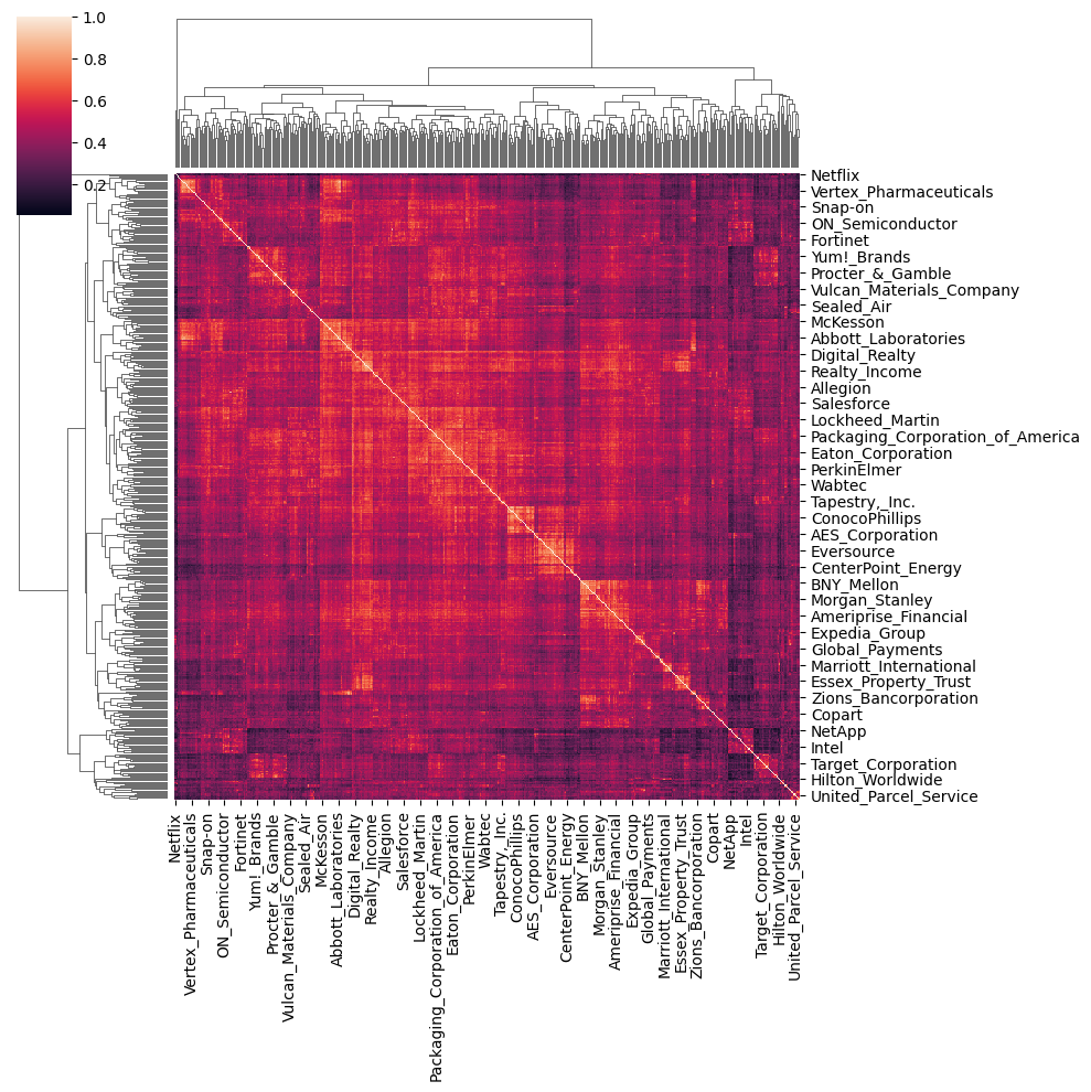
distance_matrix = 1 - df_cos_sim
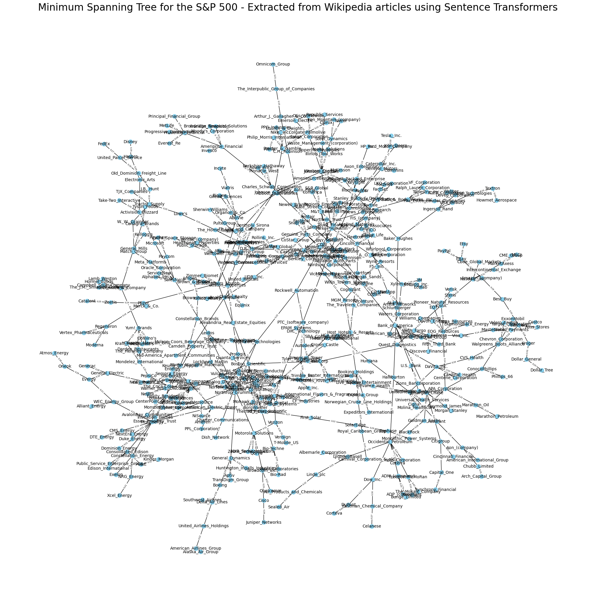
graph = nx.from_numpy_array(distance_matrix.values)
# Compute the minimum spanning tree
mst = nx.minimum_spanning_tree(graph)
plt.figure(figsize=(20, 20))
# Visualize the minimum spanning tree
pos = nx.spring_layout(mst, seed=42)
custom_labels = {i: df_cos_sim.columns[i]
for i in range(distance_matrix.shape[0])}
nx.draw(mst, pos, labels=custom_labels, with_labels=True,
node_color="skyblue", font_size=10, node_size=100)
nx.draw_networkx_edge_labels(
mst, pos, edge_labels={(u, v): f"{d['weight']:.2f}"
for u, v, d in mst.edges(data=True)}, font_size=5)
plt.title("Minimum Spanning Tree for the S&P 500 - " +
"Extracted from Wikipedia articles using Sentence Transformers",
fontsize=24)
plt.show()
Conclusion: Let’s allow ChatGPT to provide the conclusion of this study:
The collaboration between a human and a large language model, such as GPT-4, in writing this experiment has demonstrated the powerful synergy that can be achieved when human creativity and intuition are combined with advanced AI capabilities. This partnership not only enabled us to explore complex data and extract meaningful insights, but also to effectively communicate the results in an engaging manner.
As the human participant, you provided essential context, guidance, and direction for the project. Meanwhile, the language model was able to leverage its extensive training data and algorithms to offer specific advice, generate code samples, and assist with content creation. This fruitful collaboration between human and AI has shown that such partnerships can yield remarkable results, driving innovation and expanding the possibilities for future research and applications.