bivariate empirical copulas between some features

Extraction of features from a given correlation matrix

In this short blog, we extract and analyze features which should be useful for further machine learning research on financial correlation matrices, and their impact on the performance of portfolio allocation methods.

In order to describe as precisely as possible a given correlation matrix, we will extract a bunch of features from it. The features extracted and presented below are by no means exhaustive; It could be an ongoing research task to find other relevant features.

The features extracted from a given correlation matrix:

Correlation coefficients distribution (mean, std, quantiles, min, max)
Percentage of variance explained by the k-first eigenvalues, and by the eigenvalues above the Marchenko–Pastur law upper bound of its support
First eigenvector summary statistics of its entries (mean, std, quantiles, min, max)
Minimum Spanning Tree (MST) statistics based on shortest paths such as nodes’ closeness centrality, and average shortest path length
Cophenetic correlation coefficient
Condition number

These features aim at capturing several important properties of the correlation matrix:

how strong the correlation is (e.g. correlation coefficients mean, first eigenvalue),
how diverse the correlation can be (e.g. correlation coefficients std, first eigenvector std),
how hierarchical the correlation structure is (e.g. cophenetic correlation)
how complex and interconnected the system is (e.g. MST centrality quantiles and average shortest path length).

%matplotlib inline

import tensorflow as tf
from tensorflow.keras import layers
import numpy as np
import pandas as pd
from scipy.stats import rankdata
from scipy.cluster import hierarchy
from scipy.cluster.hierarchy import cophenet
from scipy.spatial.distance import squareform
import fastcluster
import networkx as nx
from statsmodels.stats.correlation_tools import corr_nearest
import matplotlib.pyplot as plt
from pprint import pprint
import warnings
warnings.filterwarnings("ignore")

def compute_mst_stats(corr):
    dist = (1 - corr) / 2
    G = nx.from_numpy_matrix(dist) 
    mst = nx.minimum_spanning_tree(G)

    features = pd.Series()
    features['mst_avg_shortest'] = nx.average_shortest_path_length(mst)


    closeness_centrality = (pd
                            .Series(list(nx
                                         .closeness_centrality(mst)
                                         .values()))
                            .describe())
    for stat in closeness_centrality.index[1:]:
        features[f'mst_centrality_{stat}'] = closeness_centrality[stat]

    return features

def compute_features_from_correl(model_corr):
    n = model_corr.shape[0]
    a, b = np.triu_indices(n, k=1)
    
    features = pd.Series()
    coefficients = model_corr[a, b].flatten()

    coeffs = pd.Series(coefficients)
    coeffs_stats = coeffs.describe()
    for stat in coeffs_stats.index[1:]:
        features[f'coeffs_{stat}'] = coeffs_stats[stat]
    features['coeffs_1%'] = coeffs.quantile(q=0.01)
    features['coeffs_99%'] = coeffs.quantile(q=0.99)
    features['coeffs_10%'] = coeffs.quantile(q=0.1)
    features['coeffs_90%'] = coeffs.quantile(q=0.9)


    # eigenvals
    eigenvals, eigenvecs = np.linalg.eig(model_corr)
    permutation = np.argsort(eigenvals)[::-1]
    eigenvals = eigenvals[permutation]
    eigenvecs = eigenvecs[:, permutation]

    pf_vector = eigenvecs[:, np.argmax(eigenvals)]
    if len(pf_vector[pf_vector < 0]) > len(pf_vector[pf_vector > 0]):
        pf_vector = -pf_vector

    features['varex_eig1'] = float(eigenvals[0] / sum(eigenvals))
    features['varex_eig_top5'] = (float(sum(eigenvals[:5])) / 
                                  float(sum(eigenvals)))
    features['varex_eig_top30'] = (float(sum(eigenvals[:30])) / 
                                   float(sum(eigenvals)))
    # Marcenko-Pastur (RMT)
    T, N = 252, n
    MP_cutoff = (1 + np.sqrt(N / T))**2
    # variance explained by eigenvals outside of the MP distribution
    features['varex_eig_MP'] = (
        float(sum([e for e in eigenvals if e > MP_cutoff])) /
        float(sum(eigenvals)))
    
    # determinant
    features['determinant'] = np.prod(eigenvals)
    
    # condition number
    features['condition_number'] = abs(eigenvals[0]) / abs(eigenvals[-1])


    # stats of the first eigenvector entries
    pf_stats = pd.Series(pf_vector).describe()
    if pf_stats['mean'] < 1e-5:
        return None
    for stat in pf_stats.index[1:]:
        features[f'pf_{stat}'] = float(pf_stats[stat])


    # stats on the MST
    features = pd.concat([features, compute_mst_stats(model_corr)],
                         axis=0)

    # stats on the linkage
    dist = np.sqrt(2 * (1 - model_corr))
    for algo in ['ward', 'single', 'complete', 'average']:
        Z = fastcluster.linkage(dist[a, b], method=algo)
        features[f'coph_corr_{algo}'] = cophenet(Z, dist[a, b])[0]

    return features.sort_index()

def compute_dataset_features(mats):
    all_features = []
    for i in range(mats.shape[0]):
        model_corr = mats[i, :, :]

        features = compute_features_from_correl(model_corr)

        if features is not None:
            all_features.append(features)
    
    return pd.concat(all_features, axis=1).T

empirical_matrices = np.load('empirical_matrices.npy')

empirical_features = compute_dataset_features(empirical_matrices)

empirical_features.describe()

	coeffs_1%	coeffs_10%	coeffs_25%	coeffs_50%	coeffs_75%	coeffs_90%	coeffs_99%	coeffs_max	coeffs_mean	coeffs_min	...	pf_50%	pf_75%	pf_max	pf_mean	pf_min	pf_std	varex_eig1	varex_eig_MP	varex_eig_top30	varex_eig_top5
count	12891.000000	12891.000000	12891.000000	12891.000000	12891.000000	12891.000000	12891.000000	12891.000000	12891.000000	12891.000000	...	12891.000000	12891.000000	12891.000000	12891.000000	12891.000000	12891.000000	12891.000000	12891.000000	12891.000000	12891.000000
mean	0.054865	0.184411	0.264647	0.356179	0.448569	0.531201	0.700261	0.874302	0.358057	-0.089366	...	0.110770	0.126837	0.156850	0.109116	0.041524	0.024270	0.382988	0.480616	0.828517	0.531707
std	0.047041	0.040486	0.040228	0.042382	0.044854	0.044363	0.048454	0.053124	0.041174	0.068130	...	0.002337	0.002334	0.010262	0.000806	0.018888	0.003405	0.038898	0.053317	0.022588	0.045089
min	-0.075686	0.067423	0.161115	0.248824	0.333421	0.407398	0.568512	0.701887	0.253199	-0.434796	...	0.101091	0.120563	0.132653	0.105851	-0.013173	0.015613	0.282363	0.347589	0.774585	0.418860
25%	0.023608	0.154149	0.232951	0.319178	0.407672	0.490917	0.664318	0.845152	0.320765	-0.130853	...	0.109250	0.125186	0.148888	0.108777	0.032930	0.021888	0.347375	0.441489	0.808563	0.491254
50%	0.059947	0.193395	0.275288	0.369782	0.463803	0.545349	0.706162	0.875702	0.371842	-0.086075	...	0.111013	0.126754	0.153498	0.109329	0.045446	0.023541	0.395434	0.501268	0.837241	0.549811
75%	0.090520	0.213517	0.294335	0.388720	0.483635	0.565356	0.738564	0.905739	0.390152	-0.042052	...	0.112485	0.128265	0.164144	0.109667	0.056018	0.025999	0.413230	0.520113	0.845770	0.566177
max	0.228811	0.409144	0.504890	0.585560	0.658309	0.715057	0.812516	0.993614	0.572143	0.099364	...	0.116784	0.135568	0.196415	0.110722	0.074222	0.036221	0.588636	0.616759	0.883207	0.674428

8 rows × 36 columns

We save the features for future use.

empirical_features.to_hdf('empirical_features.h5', key='features')

Some EDA on the features. Plotting their distribution:

plt.figure(figsize=(16, 32))
for idx, col in enumerate(empirical_features.columns):
    plt.subplot(9, 4, idx + 1)
    qlow = empirical_features[col].quantile(0.01)
    qhigh = empirical_features[col].quantile(0.99)
    plt.hist(empirical_features[col]
             .clip(lower=qlow, upper=qhigh)
             .replace(qlow, np.nan)
             .replace(qhigh, np.nan),
             bins=100, log=False)
    plt.axvline(x=empirical_features[col].mean(), color='r',
                linestyle='dashed', linewidth=2)
    plt.title(col)
plt.show()

distributions of the features

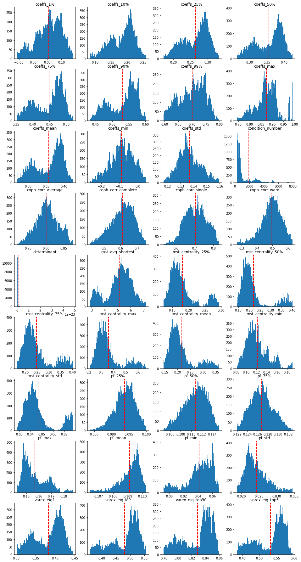
We notice two modes in the correlation coefficients distributions: probably two market regimes in the data; also in the variance explained distributions (since the percentage of variance explained by the first PCA component and the average (absolute) correlation is the same thing). These two modes can also be found in the MST statistics distributions. The condition number and determinant have a distribution which is heavily right-skewed (with some outliers). Be careful with basic linear regressions if using those two.

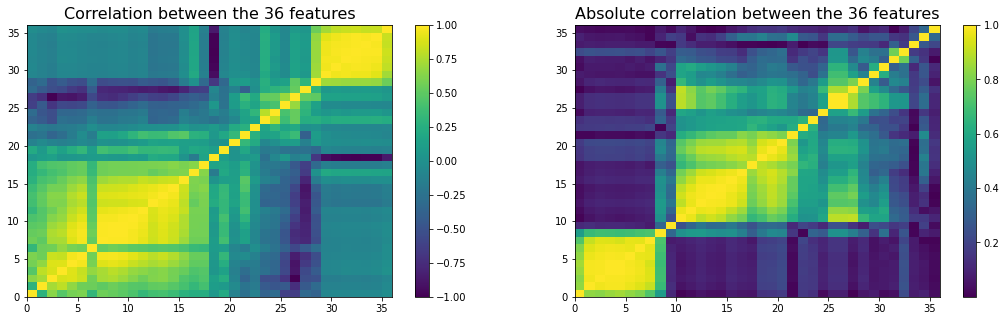
Also, many of these variables must be highly correlated because of

1) their construction (similar summary statistics, e.g. different quantiles), 2) the mathematical relations holding for PSD matrices, and general linear algebra (e.g. PCA and average correlation, determinant and condition number).

The potentially high correlation between features can make it hard to fit and interpret regression models:

estimation is more difficult in the presence of multicollinearity,
feature importance is more complex since the importance is diluted amongst the many noisy copy of the essentially same variable.

We display a re-ordered correlation matrix of the features below:

n = len(empirical_features.columns)
a, b = np.triu_indices(n, k=1)

plt.figure(figsize=(18, 5))
plt.subplot(1, 2, 1)
corr_features = empirical_features.corr(method='spearman')
dist = (1 - corr_features).values
Z = fastcluster.linkage(dist[a, b], method='ward')
permutation = hierarchy.leaves_list(
    hierarchy.optimal_leaf_ordering(Z, dist[a, b]))

sorted_corr_features = empirical_features[
    empirical_features.columns[permutation]].corr(method='spearman')
plt.pcolormesh(sorted_corr_features)
plt.colorbar()
plt.title(f'Correlation between the {n} features', fontsize=16)
plt.subplot(1, 2, 2)
corr_features = (empirical_features
                 .corr(method='spearman')
                 .abs())
dist = (1 - corr_features).values
Z = fastcluster.linkage(dist[a, b], method='ward')
permutation = hierarchy.leaves_list(
    hierarchy.optimal_leaf_ordering(Z, dist[a, b]))

sorted_corr_features = (empirical_features[
    empirical_features.columns[permutation]]
                        .corr(method='spearman')
                        .abs())
plt.pcolormesh(sorted_corr_features)
plt.colorbar()
plt.title(f'Absolute correlation between the {n} features', fontsize=16)
plt.show()

correlations between the features

nb_clusters = 4

dist = 1 - sorted_corr_features.values
dim = len(dist)
tri_a, tri_b = np.triu_indices(dim, k=1)
Z = fastcluster.linkage(dist[tri_a, tri_b], method='ward')
clustering_inds = hierarchy.fcluster(Z, nb_clusters,
                                     criterion='maxclust')
clusters = {i: [] for i in range(min(clustering_inds),
                                 max(clustering_inds) + 1)}
for i, v in enumerate(clustering_inds):
    clusters[v].append(i)
    
plt.figure(figsize=(5, 5))
plt.pcolormesh(sorted_corr_features)
for cluster_id, cluster in clusters.items():
    xmin, xmax = min(cluster), max(cluster)
    ymin, ymax = min(cluster), max(cluster)
    
    plt.axvline(x=xmin,
                ymin=ymin / dim, ymax=(ymax + 1) / dim,
                color='r')
    plt.axvline(x=xmax + 1,
                ymin=ymin / dim, ymax=(ymax + 1) / dim,
                color='r')
    plt.axhline(y=ymin,
                xmin=xmin / dim, xmax=(xmax + 1) / dim,
                color='r')
    plt.axhline(y=ymax + 1,
                xmin=xmin / dim, xmax=(xmax + 1) / dim,
                color='r')
plt.show()

for i, cluster in enumerate(clusters):
    print('Cluster', i + 1)
    cluster_members = [sorted_corr_features.index[ind]
                       for ind in clusters[cluster]]
    print('Cluster size:', len(cluster_members))
    pprint(cluster_members)
    print()

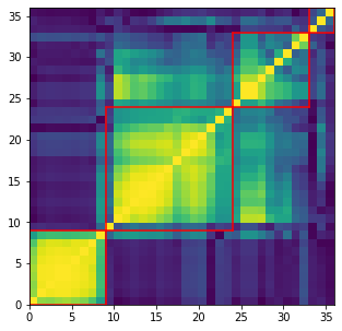
correlation matrix between the features and clusters

Cluster 1
Cluster size: 9
['mst_centrality_min',
 'mst_centrality_25%',
 'mst_centrality_50%',
 'mst_centrality_mean',
 'mst_avg_shortest',
 'mst_centrality_max',
 'mst_centrality_75%',
 'mst_centrality_std',
 'pf_max']

Cluster 2
Cluster size: 15
['pf_50%',
 'coeffs_10%',
 'coeffs_25%',
 'coeffs_50%',
 'coeffs_mean',
 'varex_eig1',
 'coeffs_75%',
 'coeffs_90%',
 'determinant',
 'varex_eig_top30',
 'varex_eig_top5',
 'varex_eig_MP',
 'coeffs_99%',
 'condition_number',
 'coeffs_max']

Cluster 3
Cluster size: 3
['coph_corr_complete', 'coeffs_std', 'coph_corr_ward']

Cluster 4
Cluster size: 9
['coeffs_min',
 'pf_mean',
 'pf_std',
 'coeffs_1%',
 'pf_min',
 'pf_75%',
 'pf_25%',
 'coph_corr_average',
 'coph_corr_single']

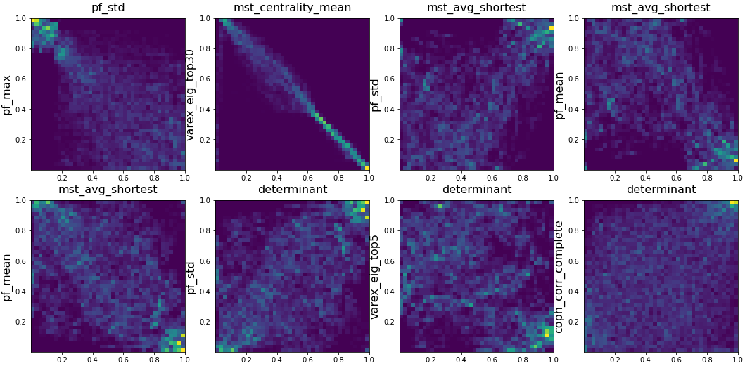
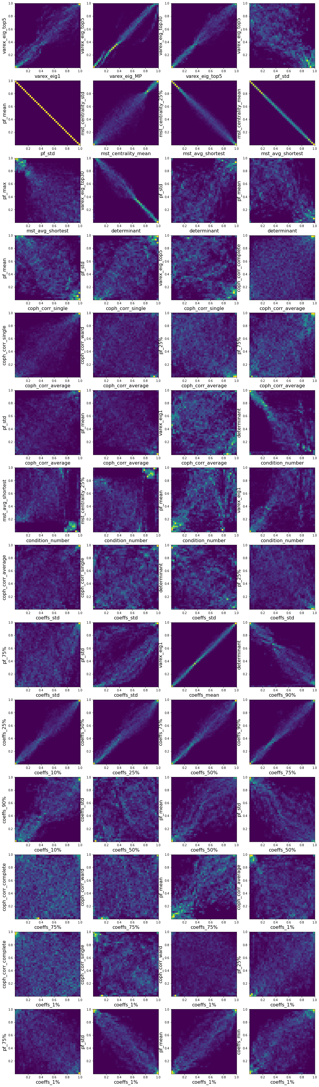
I also quickly visualized the 36*35/2 = 630 bivariate empirical copulas, and report below some interesting relations between the variables:

pairs = [('varex_eig1', 'varex_eig_top5'),
         ('varex_eig_MP', 'varex_eig_top5'),
         ('varex_eig_top5', 'varex_eig_top30'),
         ('pf_std', 'varex_eig_top5'),
         ('pf_std', 'pf_mean'),
         ('mst_centrality_mean', 'mst_centrality_std'),
         ('mst_avg_shortest', 'mst_centrality_25%'),
         ('mst_avg_shortest', 'mst_centrality_mean'),
         ('mst_avg_shortest', 'pf_max'),
         ('determinant', 'varex_eig_top30'),
         ('determinant', 'pf_std'),
         ('determinant', 'pf_mean'),
         ('coph_corr_single', 'pf_mean'),
         ('coph_corr_single', 'pf_std'),
         ('coph_corr_single', 'varex_eig_top5'),
         ('coph_corr_average', 'coph_corr_complete'),
         ('coph_corr_average', 'coph_corr_single'),
         ('coph_corr_average', 'coph_corr_ward'),
         ('coph_corr_average', 'pf_25%'),
         ('coph_corr_average', 'pf_75%'),
         ('coph_corr_average', 'pf_std'),
         ('coph_corr_average', 'pf_mean'),
         ('coph_corr_average', 'varex_eig1'),
         ('condition_number', 'determinant'),
         ('condition_number', 'mst_avg_shortest'),
         ('condition_number', 'mst_centrality_25%'),
         ('condition_number', 'pf_mean'),
         ('condition_number', 'varex_eig1'),
         ('coeffs_std', 'coph_corr_average'),
         ('coeffs_std', 'coph_corr_single'),
         ('coeffs_std', 'determinant'),
         ('coeffs_std', 'pf_25%'),
         ('coeffs_std', 'pf_75%'),
         ('coeffs_std', 'pf_std'),
         ('coeffs_mean', 'varex_eig1'),
         ('coeffs_90%', 'determinant'),
         ('coeffs_10%', 'coeffs_25%'),
         ('coeffs_25%', 'coeffs_50%'),
         ('coeffs_50%', 'coeffs_75%'),
         ('coeffs_75%', 'coeffs_90%'),
         ('coeffs_10%', 'coeffs_90%'),
         ('coeffs_50%', 'coeffs_std'),
         ('coeffs_50%', 'pf_mean'),
         ('coeffs_50%', 'pf_std'),
         ('coeffs_75%', 'coph_corr_complete'),
         ('coeffs_75%', 'coph_corr_ward'),
         ('coeffs_75%', 'pf_mean'),
         ('coeffs_1%', 'coph_corr_average'),
         ('coeffs_1%', 'coph_corr_complete'),
         ('coeffs_1%', 'coph_corr_single'),
         ('coeffs_1%', 'coph_corr_ward'),
         ('coeffs_1%', 'pf_25%'),
         ('coeffs_1%', 'pf_75%'),
         ('coeffs_1%', 'pf_std'),
         ('coeffs_1%', 'pf_mean'),
         ('coeffs_1%', 'coeffs_min'),]

plt.figure(figsize=(18, 66))
for idx, (var1, var2) in enumerate(pairs):
    plt.subplot(14, 4, idx + 1)
    rk1 = rankdata(empirical_features[var1])
    rk1 /= len(rk1)
    rk2 = rankdata(empirical_features[var2])
    rk2 /= len(rk2)
    plt.hist2d(rk1, rk2, bins=40)
    plt.xlabel(var1, fontsize=16)
    plt.ylabel(var2, fontsize=16)
plt.show()

empirical bivariate copulas between the features

You can download the features here.