[Paper + Implementation] Hierarchical PCA and Applications to Portfolio Management
[Paper + Implementation] Hierarchical PCA and Applications to Portfolio Management
First thoughts after reading Hierarchical PCA and Applications to Portfolio Management by Marco Avellaneda.
-
PCA and $k$-means have a theoretical connection, described in this old ICML paper (2004): $K$-means Clustering via Principal Component Analysis; However, as the paper is rather sloppy, I would suggest to read as well this Cross Validated question What is the relation between $k$-means clustering and PCA? related to it, where there is a detailed and clear answer.
-
Can we establish something similar between hierarchical PCA (HPCA) and hierarchical clustering, say with the Ward algorithm?
-
We can use hierarchical clustering to define the hierarchical “layers” of the HPCA, i.e. extract several meaningful nested partitions (the “layers”) from the dendrogram.
-
One might want to use Estimation of Theory-Implied Correlation Matrices by Marcos Lopez de Prado to tilt the statistical clusters toward official sectors (say GICS) if it is a wanted property (as it seems to be in the paper), otherwise to something else?
%matplotlib inline

import pandas as pd
import numpy as np
import fastcluster
from scipy.cluster import hierarchy
from sklearn.linear_model import LinearRegression
import matplotlib.pyplot as plt
import plotly.graph_objects as go
Load and prepare data
df = pd.read_csv('data/SP500_HistoTimeSeries.csv')
df = df.set_index('Date')
df.index = pd.to_datetime(df.index)
df = df.sort_index()
del df['SPX Index']
returns = df.pct_change()
stock_features = pd.read_csv('data/stock_features.csv')
stock_features = stock_features[['Unnamed: 1',
                                 'INDUSTRY_SECTOR',
                                 'INDUSTRY_GROUP',
                                 'INDUSTRY_SUBGROUP']]
stock_features.columns = ['ticker'] + list(stock_features.columns[1:])
industry_info = [(row[1]['ticker'].split(' ')[0],
                  row[1]['INDUSTRY_SECTOR'],
                  row[1]['INDUSTRY_GROUP'],
                  row[1]['INDUSTRY_SUBGROUP'])
                 for row in stock_features.iterrows()]
industry_info = [e for e in industry_info
                 if 'Invalid Security' not in e[1]]
industry_permutation = sorted(industry_info,
                              key=lambda x: (x[1], x[2], x[3]))
industry_tickers = [e[0] for e in industry_permutation]

ticker2sector = {e[0]: e[1] for e in industry_permutation}
ticker2group = {e[0]: e[2] for e in industry_permutation}
industry_permutation[:5]
[('CF', 'Basic Materials', 'Chemicals', 'Agricultural Chemicals'),
 ('IPI', 'Basic Materials', 'Chemicals', 'Agricultural Chemicals'),
 ('MON', 'Basic Materials', 'Chemicals', 'Agricultural Chemicals'),
 ('MOS', 'Basic Materials', 'Chemicals', 'Agricultural Chemicals'),
 ('RTK', 'Basic Materials', 'Chemicals', 'Agricultural Chemicals')]
industry_permutation[-5:]
[('CWT', 'Utilities', 'Water', 'Water'),
 ('MSEX', 'Utilities', 'Water', 'Water'),
 ('SJW', 'Utilities', 'Water', 'Water'),
 ('WTR', 'Utilities', 'Water', 'Water'),
 ('YORW', 'Utilities', 'Water', 'Water')]
recent_returns = returns.iloc[-252 * 2:]
short_names = [n.split(' ')[0]
               for n in recent_returns.columns]
recent_returns.columns = short_names
recent_returns.shape
(504, 505)
# standardized returns
recent_returns = ((recent_returns - recent_returns.mean(axis=0)) /
                  recent_returns.std(axis=0))
for col in recent_returns:
    try:
        if (len(recent_returns[col].dropna()) <
            len(recent_returns[col])):
            del recent_returns[col]
        if col not in industry_tickers:
            del recent_returns[col]
    except:
        pass

# alone in the Diversified GIC sector
del recent_returns['LUK']

recent_returns.shape
(504, 490)
industry_tickers = [e for e in industry_tickers
                    if e in recent_returns.columns]
Input: Full empirical correlation matrix
plt.figure(figsize=(18, 5))

# arbitrary order
corr_returns = recent_returns.corr()

plt.subplot(1, 3, 1)
plt.pcolormesh(corr_returns)
plt.colorbar()
plt.title('Correlation matrix with arbitrary order')

# sorted by alphabetically by industry sector, group, subgroup
industry_corr = recent_returns[industry_tickers].corr()

plt.subplot(1, 3, 2)
plt.pcolormesh(industry_corr)
plt.colorbar()
plt.title('Correlation matrix with industry order')


# sorted by hierarchical clustering
dist = 1 - corr_returns.values
dim = len(dist)
tri_a, tri_b = np.triu_indices(dim, k=1)
Z = fastcluster.linkage(dist[tri_a, tri_b], method='ward')
permutation = hierarchy.leaves_list(
    hierarchy.optimal_leaf_ordering(Z, dist[tri_a, tri_b]))
HC_tickers = recent_returns.columns[permutation]
HC_corr = corr_returns.values[permutation, :][:, permutation]

plt.subplot(1, 3, 3)
plt.pcolormesh(HC_corr)
plt.colorbar()
plt.title('Correlation matrix with HC-induced order')
plt.show()
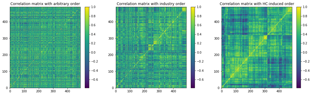
Note that in the paper, the author is using the GIC sectors to order the stocks (center), we can see that we can find a better ordering with a hierarchical clustering (right). In the following, we will use both the GICS (as in the author paper), and clusters extracted from the hierarchical clustering (which may be an improvement on the author’s original method).
Defining the 9 GIC Sectors, and the 9 clusters
Let’s group the stocks into their respective sectors:
industry_classification = {}
for e in industry_permutation:
    if e[0] in industry_tickers:
        if e[1] not in industry_classification:
            industry_classification[e[1]] = [e[0]]
        else:
            industry_classification[e[1]].append(e[0])
for sector in industry_classification:
    print(sector)
    print('sector size:', len(industry_classification[sector]))
    print()
Basic Materials
sector size: 19

Communications
sector size: 34

Consumer, Cyclical
sector size: 74

Consumer, Non-cyclical
sector size: 99

Energy
sector size: 38

Financial
sector size: 91

Industrial
sector size: 64

Technology
sector size: 43

Utilities
sector size: 28
Let’s group the stocks into their respective clusters:
nb_clusters = 9

dist = 1 - HC_corr
dim = len(dist)
tri_a, tri_b = np.triu_indices(dim, k=1)
Z = fastcluster.linkage(dist[tri_a, tri_b], method='ward')
clustering_inds = hierarchy.fcluster(Z, nb_clusters,
                                     criterion='maxclust')
clusters = {i: [] for i in range(min(clustering_inds),
                                 max(clustering_inds) + 1)}
for i, v in enumerate(clustering_inds):
    clusters[v].append(i)

plt.figure(figsize=(5, 5))
plt.pcolormesh(HC_corr)
for cluster_id, cluster in clusters.items():
    xmin, xmax = min(cluster), max(cluster)
    ymin, ymax = min(cluster), max(cluster)

    plt.axvline(x=xmin,
                ymin=ymin / dim, ymax=(ymax + 1) / dim,
                color='r')
    plt.axvline(x=xmax + 1,
                ymin=ymin / dim, ymax=(ymax + 1) / dim,
                color='r')
    plt.axhline(y=ymin,
                xmin=xmin / dim, xmax=(xmax + 1) / dim,
                color='r')
    plt.axhline(y=ymax + 1,
                xmin=xmin / dim, xmax=(xmax + 1) / dim,
                color='r')
plt.show()

for i, cluster in enumerate(clusters):
    print('Cluster', i + 1)
    print(len([HC_tickers[ind] for ind in clusters[cluster]]))
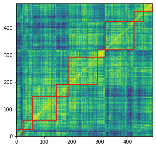
Cluster 1
25
Cluster 2
45
Cluster 3
35
Cluster 4
85
Cluster 5
27
Cluster 6
102
Cluster 7
104
Cluster 8
31
Cluster 9
36
Let’s compare the industry classification, and the clustering classification. Using a Sankey diagram, it is very easy to visualize their differences. It can be applied more generally to compare hierarchical classifications (cf. this short paper about the HCMapper tool).
label_GICS = list(industry_classification.keys())
label_clusters = ['Cluster {}'.format(i + 1) for i in range(9)]
labels = label_GICS + label_clusters
sources = []
targets = []
values = []
for label_source in label_GICS:
    for label_target in label_clusters:
        intersection = set(industry_classification[label_source]).intersection(
            [HC_tickers[ind]
             for ind in clusters[int(label_target.split(' ')[1])]])

        if intersection:
            sources.append(labels.index(label_source))
            targets.append(labels.index(label_target))
            values.append(len(intersection))
fig = go.Figure(data=[go.Sankey(
    node=dict(
      pad=15,
      thickness=20,
      line=dict(color = "black", width = 0.5),
      label=labels,
      color="blue"),
    link=dict(
      source=sources,
      target=targets,
      value=values))])

fig.update_layout(title_text="GICS vs. Clusters", font_size=10)
fig.show()
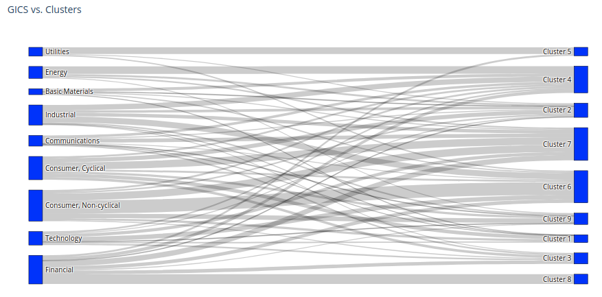
Except for Cluster 5 which is matching the Utilities sector quite closely, and Cluster 8 which contains only Financial companies, clusters obtained are quite different from the sectors as defined by the GICS (or BICS actually… paper is using GICS) classification.
The Hierarchical PCA (HPCA) assumption
The HPCA assumption is:
If sector(i) $\neq$ sector(j), then $Corr(\epsilon_i, \epsilon_j) = 0$,
where $\epsilon_i, \epsilon_j$ are residuals of the model $X_i = \beta_i F^{(1,~\text{sector}(i))} + \epsilon_i$, $\beta_i$ being the regression coefficient of the returns of asset $i$ on the first factor of sector$(i)$.
Let’s check how realistic this assumption is.
We will compute the first eigenvalue $\lambda$, first eigenvector $V$, and first eigenportfolio $F$ for each sector.
Then, we will compute for each stock $i$ the residual $\epsilon_i = X_i - \beta_i F$.
Finally, we will check the distribution of the correlation coefficients $c_{ij} = Corr(\epsilon_i, \epsilon_j)$ of residuals $\epsilon_i, \epsilon_j$ for stocks $i$ and $j$ not belonging to the same sector.
eigen_sectors = {}

for sector in industry_classification:
    tickers = industry_classification[sector]
    corr_sector = corr_returns.loc[tickers][tickers]
    rets_sector = recent_returns[tickers]

    eigenvals, eigenvecs = np.linalg.eig(corr_sector.values)

    idx = eigenvals.argsort()[::-1]
    eigenvals = eigenvals[idx]
    eigenvecs = eigenvecs[:, idx]

    val1 = eigenvals[0]
    vec1 = eigenvecs[:, 0]
    F1 = (1 / np.sqrt(val1)) * np.multiply(
        vec1, rets_sector.values).sum(axis=1)

    eigen_sectors[sector] = {
        'tickers': tickers,
        'val1': val1,
        'vec1': vec1,
        'F1': F1,
    }
betas = {}
residuals = {}
for ticker in recent_returns.columns:

    ticker_rets = recent_returns[ticker]
    sector_F1 = eigen_sectors[ticker2sector[ticker]]['F1']

    reg = LinearRegression(fit_intercept=False).fit(
        sector_F1.reshape(-1, 1), ticker_rets)

    beta = reg.coef_[0]

    betas[ticker] = beta
    residuals[ticker] = ticker_rets - beta * sector_F1
correl_residuals = []
for ticker1 in recent_returns.columns:
    for ticker2 in recent_returns.columns:
        if ticker2sector[ticker1] != ticker2sector[ticker2]:
            correl_residuals.append(
                np.corrcoef(residuals[ticker1],
                            residuals[ticker2])[0, 1])
len(correl_residuals)
206852
plt.figure(figsize=(16, 5))
plt.subplot(1, 2, 1)
plt.hist(correl_residuals, bins=100,
         alpha=0.5, density=True, log=False)
plt.axvline(x=np.mean(correl_residuals),
            color='b', linestyle='dashed', linewidth=2)
plt.title('Correlations of inter sector residuals')
plt.subplot(1, 2, 2)
plt.hist(correl_residuals, bins=100,
         alpha=0.5, density=True, log=True)
plt.axvline(x=np.mean(correl_residuals),
            color='b', linestyle='dashed', linewidth=2)
plt.title('Correlations of inter sector residuals (log density)')
plt.show()
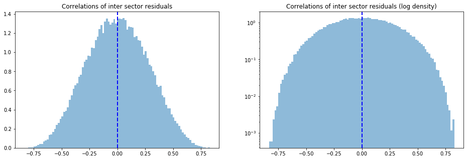
Note that the average correlation of the inter sector residuals is 0, and is normally distributed around 0 with a standard deviation of 27%.
The Hierarchical PCA correlation matrix
The Hierarchical PCA (HPCA) consists essentially in applying a PCA on a modified correlation matrix.
The full empirical correlation matrix is modified such that the inter sector correlation is essentially the correlation between the first eigenvector of the sectors. Intra sector correlation is left unchanged.
The HPCA assumption, i.e. if sector(i) $\neq$ sector(j), then $Corr(\epsilon_i, \epsilon_j) = 0$, justifies the definition of a transformed correlation matrix, the HPCA correlation matrix:
-
If sector$(i)$ = sector$(j)$, $\tilde{R}_{ij} = R_{ij}$,
-
If sector$(i)$ $\neq$ sector$(j)$, $\tilde{R}_{ij} = \beta_i \beta_j Corr(F^{(1,~\text{sector}(i))}, F^{(1,~\text{sector}(j))})$.
Author proves that $\tilde{R}$ is indeed a valid correlation matrix.
Let’s compute the HPCA correlation matrix:
# ordered following industry_tickers
HPCA_corr = industry_corr.copy()
for ticker1 in HPCA_corr.columns:
    beta_1 = betas[ticker1]
    F1_1 = eigen_sectors[ticker2sector[ticker1]]['F1']
    for ticker2 in HPCA_corr.columns:
        beta_2 = betas[ticker2]
        F1_2 = eigen_sectors[ticker2sector[ticker2]]['F1']
        if ticker2sector[ticker1] != ticker2sector[ticker2]:
            rho_sector = np.corrcoef(F1_1, F1_2)[0, 1]
            mod_rho = beta_1 * beta_2 * rho_sector
            HPCA_corr.at[ticker1, ticker2] = mod_rho
            HPCA_corr.at[ticker2, ticker1] = mod_rho
# sorted by alphabetically by industry sector, group, subgroup
plt.figure(figsize=(16, 6))
plt.subplot(1, 2, 1)
plt.pcolormesh(industry_corr)
plt.colorbar()
plt.title('Correlation matrix with industry order')

plt.subplot(1, 2, 2)
plt.pcolormesh(HPCA_corr)
plt.colorbar()
plt.title('HPCA correlation matrix with industry order')
plt.show()
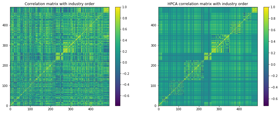
We observe that the intra sector correlations are as noisy as in the original correlation matrix, but some noise has been filtered out of the inter sector correlations.
Why didn’t the author also process the intra sector correlations?
HPCA vs. PCA
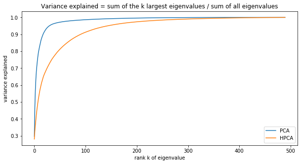
Let’s compare the eigenvalues and eigenvectors of the HPCA and the PCA.
eigenvals, eigenvecs = np.linalg.eig(industry_corr.values)

idx = eigenvals.argsort()[::-1]
pca_eigenvals = eigenvals[idx]
pca_eigenvecs = eigenvecs[:, idx]

eigenvals, eigenvecs = np.linalg.eig(HPCA_corr.values)

idx = eigenvals.argsort()[::-1]
hpca_eigenvals = eigenvals[idx]
hpca_eigenvecs = eigenvecs[:, idx]
plt.figure(figsize=(10, 5))
plt.plot(np.cumsum(pca_eigenvals) / pca_eigenvals.sum(), label='PCA')
plt.plot(np.cumsum(hpca_eigenvals) / hpca_eigenvals.sum(), label='HPCA')
plt.xlabel('rank k of eigenvalue')
plt.ylabel('variance explained')
plt.title('Variance explained = ' +
          'sum of the k largest eigenvalues / sum of all eigenvalues')
plt.legend()
plt.show()
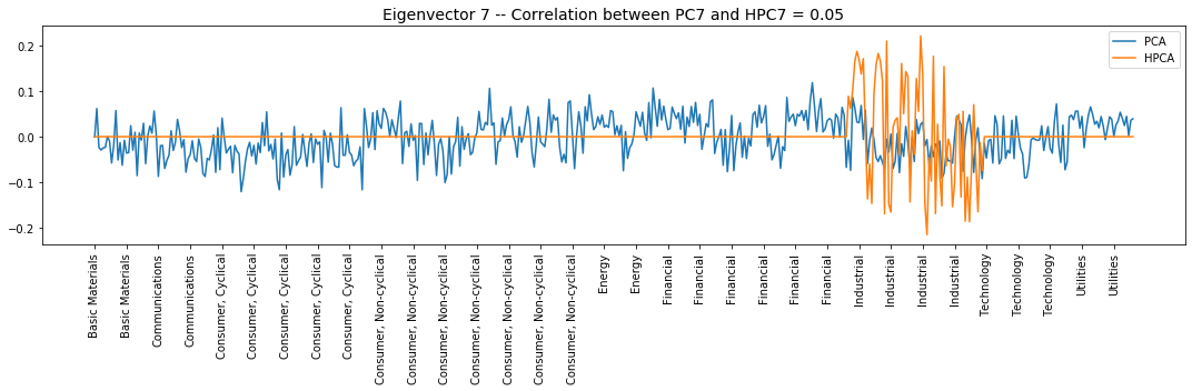
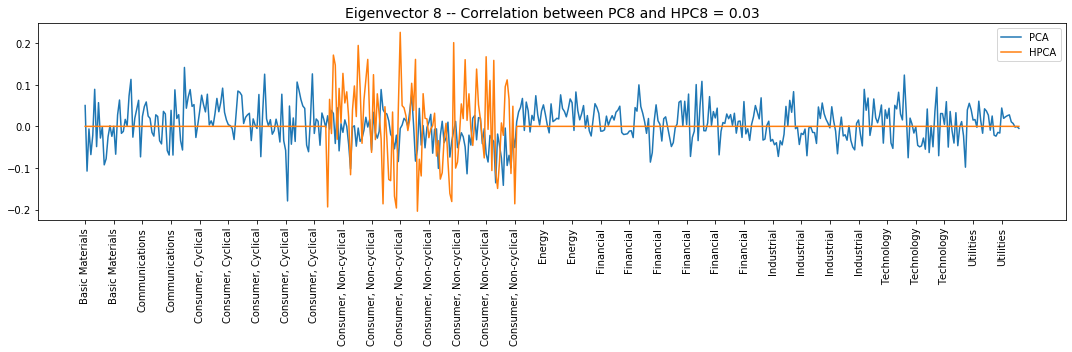
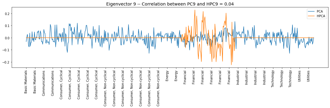
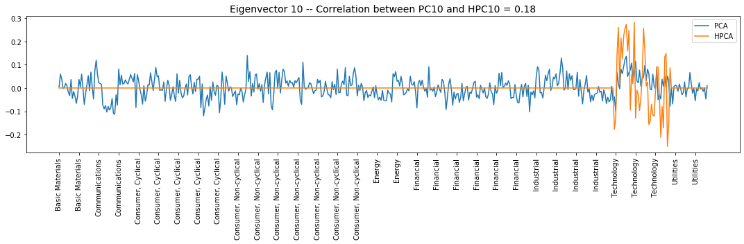
for i in range(10):
fig, ax = plt.subplots(figsize=(15, 5),
tight_layout=True)
corr_pcs = np.corrcoef(pca_eigenvecs[:, i],
hpca_eigenvecs[:, i])[0, 1]
if corr_pcs < 0:
hpca_eigenvecs[:, i] = -hpca_eigenvecs[:, i]
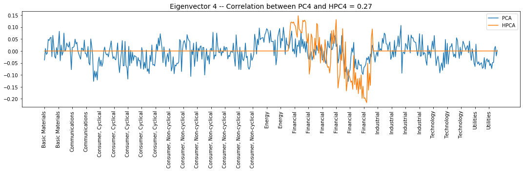
plt.plot(pca_eigenvecs[:, i], label='PCA')
plt.plot(hpca_eigenvecs[:, i], label='HPCA')
plt.title('Eigenvector {} -- ' +
'Correlation between PC{} and HPC{} = {}'.format(
i + 1, i + 1, i + 1, round(abs(corr_pcs), 2)), fontsize=14)
spacing = 15
xticks = [ticker2sector[tk] for itk, tk in enumerate(industry_tickers)
if itk % spacing == 0]
xorig = [ix for ix in range(len(industry_tickers))
if ix % spacing == 0]
plt.xticks(xorig, xticks)
ax.tick_params(axis='x', rotation=90)
plt.legend()
plt.show()
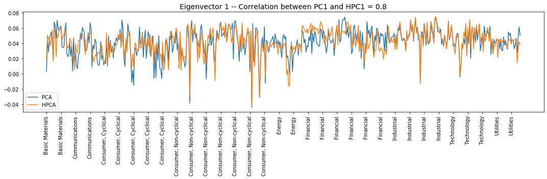
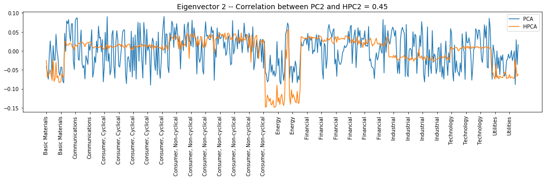
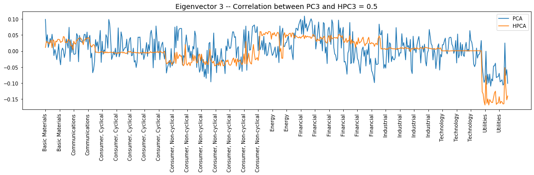
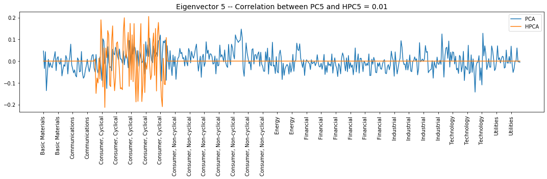
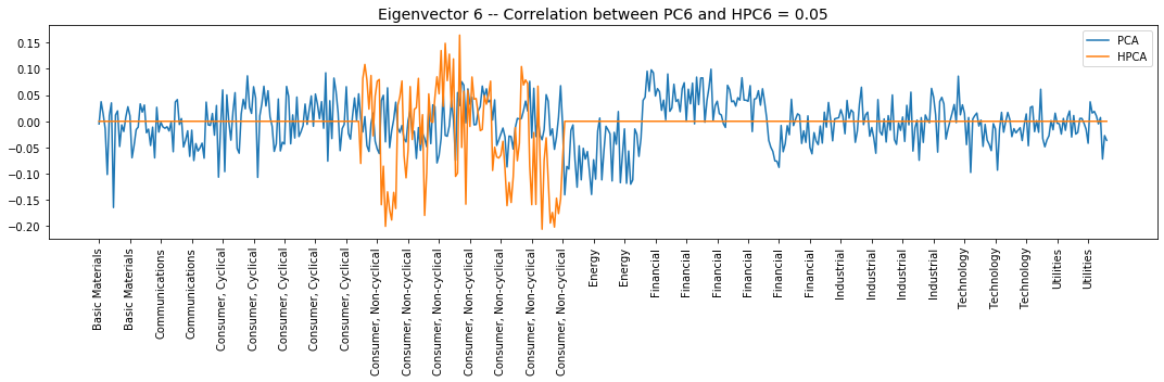
Interpretation of the eigenvectors:
-
Eigenvector 1: The market
-
Eigenvector 2: Basic Materials, Energy, and Utilities
-
Eigenvector 3: Utilities
-
Eigenvector 4: Financial, Long/Short Banks vs. Insurance & REITS
-
Eigenvector 5: L/S in the Consumer, Cyclical
-
Eigenvector 6: L/S in the Consumer, Non-cyclical
-
Eigenvector 7: L/S in the Industrial
-
Eigenvector 8: Another L/S in the Consumer, Non-cyclical
-
Eigenvector 9: L/S within the Financial
-
Eigenvector 10: Technology, Long/Short Computers & Semiconductors vs. Software
Analysis of residuals via Random Matrix Theory
rank_cutoff = 50
def compute_eigen(input_matrix, rank_cutoff=30):

    eigenvals, eigenvecs = np.linalg.eig(input_matrix.values)

    idx = eigenvals.argsort()[::-1]
    eigenvals = eigenvals[idx]
    eigenvecs = eigenvecs[:, idx]

    vals = []
    vecs = []
    Fs = []
    for k in range(rank_cutoff):
        val_k = eigenvals[k]
        vec_k = eigenvecs[:, k]
        F_k = (1 / np.sqrt(val_k)) * np.multiply(
            vec_k, recent_returns[industry_tickers].values).sum(axis=1)
        vals.append(val_k)
        vecs.append(vec_k)
        Fs.append(F_k)

    eigen = {
        'tickers': industry_tickers,
        'vals': vals,
        'vecs': vecs,
        'Fs': Fs,
    }

    return eigen

def compute_residuals(ticker, factors):
    ticker_rets = recent_returns[ticker]
    reg = LinearRegression(fit_intercept=False).fit(
        factors.T, ticker_rets)
    betas = reg.coef_

    return (ticker_rets -
            np.multiply(betas, factors.T).sum(axis=1))

def compute_all_residuals(input_corr):
    all_tickers = input_corr.columns
    eigen = compute_eigen(input_corr)
    residuals = {}
    for ticker in all_tickers:
        residuals[ticker] = compute_residuals(
            ticker, np.array(eigen['Fs']))

    return residuals
pca_residuals = compute_all_residuals(industry_corr)
hpca_residuals = compute_all_residuals(HPCA_corr)
def compute_correl_residuals(residuals):
    residuals_correls = np.ones(industry_corr.shape)
    for i, ticker1 in enumerate(industry_corr.columns):
        for j, ticker2 in enumerate(industry_corr.columns):
            if j > i:
                residuals_correls[i, j] = np.corrcoef(
                    residuals[ticker1], residuals[ticker2])[0, 1]
                residuals_correls[j, i] = residuals_correls[i, j]

    return residuals_correls
pca_correl_residuals = compute_correl_residuals(pca_residuals)
hpca_correl_residuals = compute_correl_residuals(hpca_residuals)
plt.figure(figsize=(15, 5))
plt.subplot(1, 2, 1)
plt.hist(pca_correl_residuals[tri_a, tri_b],
         bins=100, alpha=0.5,
         label='PCA resid. correls')
plt.axvline(x=np.mean(pca_correl_residuals[tri_a, tri_b]),
            color='b', linewidth=2)

plt.hist(hpca_correl_residuals[tri_a, tri_b],
         bins=100, alpha=0.5,
         label='HPCA resid. correls')
plt.axvline(x=np.mean(hpca_correl_residuals[tri_a, tri_b]),
            color='r', linestyle='dashed', linewidth=2, alpha=0.8)
plt.legend()

plt.subplot(1, 2, 2)
plt.hist(pca_correl_residuals[tri_a, tri_b],
         bins=100, alpha=0.5, log=True,
         label='PCA resid. correls')
plt.axvline(x=np.mean(pca_correl_residuals[tri_a, tri_b]),
            color='b', linewidth=2)

plt.hist(hpca_correl_residuals[tri_a, tri_b],
         bins=100, alpha=0.5, log=True,
         label='HPCA resid. correls')
plt.axvline(x=np.mean(hpca_correl_residuals[tri_a, tri_b]),
            color='r', linestyle='dashed', linewidth=2, alpha=0.8)
plt.legend()

plt.show()

def get_sorted_eigens(corr):
    eigenvals, eigenvecs = np.linalg.eig(corr)

    idx = eigenvals.argsort()[::-1]
    eigenvals = eigenvals[idx]
    eigenvecs = eigenvecs[:, idx]

    return eigenvals, eigenvecs
If there were no information left in the correlation matrix of residuals, this one should have similar characteristics to a random matrix. Random Matrix Theory tells us that the eigenvalues of a pure noise matrix follow the Marcenko-Pastur distribution. This result holds asymptotically when $N \rightarrow \infty$ (the number of variables tends to infinity), $T \rightarrow \infty$ (the number of observations tends to infinity), and $N/T \rightarrow \gamma$ (a constant). However, even for $N$ in the few hundreds, small-ish random matrices exhibit a spectrum very close to the Marcenko-Pastur distribution allowing us to use this tool in practice.
plt.figure(figsize=(15, 5))
for method, corr in zip(['PCA', 'HPCA'],
                [pca_correl_residuals, hpca_correl_residuals]):
    eigenvals, eigenvecs = get_sorted_eigens(corr)

    plt.hist(eigenvals, bins=100, alpha=0.5, log=True, label=method)

# Marcenko-Pastur (RMT)
T, N = recent_returns.shape
MP_cutoff = (1 + np.sqrt(N / T))**2

random_noise = np.random.multivariate_normal(mean=[0] * N,
                                             cov=np.diag([1] * N),
                                             size=T)
random_corr = np.corrcoef(random_noise.T)
eigenvals, eigenvecs = get_sorted_eigens(random_corr)
plt.hist(eigenvals, bins=100, alpha=0.5, log=True, label='MP')

plt.axvline(x=MP_cutoff, label='MP cutoff',
            color='r', linestyle='dashed', linewidth=2, alpha=0.8)
plt.legend()
plt.show()
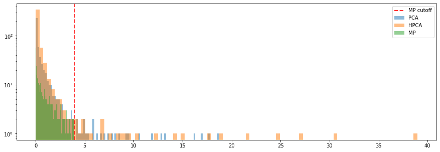
It seems that it still remains a bit of information in the residuals of the HPCA model (considering the first 50 eigenvectors), less for the PCA. It is consistent with the growth in explained variance for each model: For a given level of explained variance, less eigenvectors are needed for PCA than for HPCA. Here, since we took the same number of eigenvectors, PCA can explain more variance, and thus residuals are more noisy than for HPCA.
Conclusion: We have implemented the HPCA model, and compared it to the standard PCA. We were able to replicate the results exposed in the paper. After these first experiments, we think there is room to improve the methodology.
In future experiments, we will explore the potential benefits of using a hierarchical clustering instead of a simple GICS classification. Also, as in the paper, we only did one hierarchical layer, but using hierarchical clustering, it would be very easy to extend to more layers.
Another venue of exploration is to study the similarities between this PCA which is tilted by some external information such as a classification (or a hierarchical classification), and the Theory-Implied Correlation Matrices by Marcos Lopez de Prado which essentially blend a dendrogram obtained via hierarchical clustering and a given hierarchical classification (e.g. GICS). So, the latter technique is also tilting a Hierarchical Clustering with some external information.
Given the mathematical relations between PCA and $k$-means, it would be interesting to dig further into the potential mathematical ties between Hierarchical PCA and Hierarchical Clustering, or the Theory-Implied Correlation Matrices by Marcos Lopez de Prado.