Disentangling Speech Embeddings: Removing Text Content from Audio Embeddings with Regression

Disentangling Speech Embeddings: Removing Text Content from Audio Embeddings with Regression
tl;dr: Speech embeddings encode both text content and audio-specific features (e.g., speaker identity, prosody). This blog explores how to disentangle these components by using Ridge regression to remove text content, leaving residual embeddings that focus on speaker-specific characteristics. We analyze these residual embeddings, and find that the residuals effectively isolate audio features.
Table of Contents
- Introduction
- Data Preparation
- Residualizing Audio Embeddings via Regression
- Analyzing Embedding Similarities
- Discussion and Conclusion
1. Introduction
Over the past few years, advances in deep learning—especially using transformer architectures and self-supervised learning—have revolutionized audio and speech processing. Modern models produce rich speech embeddings that encapsulate various aspects of the signal: background noise, speaker identity, prosody, and even the semantic content (i.e., what is being said).
However, if you plan to use these embeddings for downstream tasks, an important question arises: What exactly is contained in these embeddings? Are they dominated by the text content, or do they also capture pure audio characteristics? In this blog post, we walk through a notebook that tackles this question by “regressing out” the text content from the audio embeddings. We then analyze both the original and residual embeddings to see how the similarity patterns change, and whether we have isolated the speaker/audio-specific features.
N.B. This blog post serves as a pedagogical introduction to the core concepts and methodologies explored in Hamdan Al Ahbabi’s PhD research as part of his doctoral studies at Khalifa University, under my co-supervision. It is entirely non-work-related and should not be interpreted as such. Instead, its purpose is to support and complement future presentations at academic conferences.
Background Concepts
Before we dive into the analysis, let’s briefly define a few key concepts:
- Embeddings: High-dimensional numerical representations of text or audio data, capturing semantic or speaker-specific information.
- Cosine Similarity: A measure of similarity between two vectors, calculated as the cosine of the angle between them. It ranges from -1 (opposite) to 1 (identical).
- Ridge Regression: A linear regression model with an L2 regularization term that prevents overfitting by penalizing large coefficients.
With these definitions in mind, let’s move on to the data preparation.
2. Data Preparation
We first load and preprocess our data. In our case, we have:
- Text embeddings (shape 1536) stored in a Parquet file.
- Audio embeddings (shape 768) stored as
.npyfiles for each sentence and voice.
2.1 Loading Audio and Text Embeddings
We start by importing our libraries and reading in the embeddings.
import numpy as np
import pandas as pd
import matplotlib.pyplot as plt
from sklearn.linear_model import Ridge
from sklearn.metrics.pairwise import cosine_similarity

# Define a list of voice labels used in the recordings.
voices = [
    "alloy", "ash", "coral", "echo", "fable", "onyx", "nova", "sage", "shimmer",
]

# Load text embeddings and sentence metadata.
text_emb = pd.read_parquet("text_embeddings.parquet")
sentences = pd.read_parquet("earnings_calls_sentences.parquet")

# Process audio embeddings: compute a single (mean-pooled) vector per recording.
audio_embeddings = []
for idx in range(len(sentences)):
    for voice in voices:
        embedding = np.load(f"audio_embeddings/speech_{idx}/speech_{voice}.npy")
        # Mean pool over the time axis; adjust indexing as needed.
        single_embedding = embedding.mean(axis=1)[0].tolist()
        audio_embeddings.append([f"{idx}_{voice}"] + single_embedding)
2.2 Experimental Setup
Our experiments start with a dataset of 52 unique sentences, each spoken by 9 different voices (e.g., “alloy,” “ash,” “coral”). This results in a total of 468 audio recordings, with each sentence-voice pair represented by:
- Text embeddings (dimensionality: 1536) encoding the semantic content of the sentence.
- Audio embeddings (dimensionality: 768) capturing both speaker-specific characteristics and the spoken content.
This setup allows us to explore how embeddings encode information across voices and sentences and how residualizing affects these representations.
2.3 Building DataFrames
Next, we construct DataFrames for the audio embeddings. For each sentence (indexed by idx) and for each voice, we load the corresponding .npy file, compute the mean over time frames, and store the result. We then repeat the text embedding for each voice (since each sentence’s text is paired with multiple voices).
# Create a DataFrame with audio embeddings and set the index.
df_audio_emb = pd.DataFrame(audio_embeddings).set_index(0)
df_audio_emb.index.name = "sent_speaker"
display(df_audio_emb.head())

# Expand the text embeddings to match the number of audio samples.
exp_text_emb = []
for idx, row in text_emb.iterrows():
    for _ in range(len(voices)):
        exp_text_emb.append(row.values.tolist())
df_text_emb = pd.DataFrame(exp_text_emb)
display(df_text_emb.head())
| 1 | 2 | 3 | 4 | 5 | 6 | 7 | 8 | 9 | 10 | ... | 759 | 760 | 761 | 762 | 763 | 764 | 765 | 766 | 767 | 768 | |
|---|---|---|---|---|---|---|---|---|---|---|---|---|---|---|---|---|---|---|---|---|---|
| sent_speaker | |||||||||||||||||||||
| 0_alloy | -0.181595 | 0.044399 | 0.336770 | 0.053689 | 0.187663 | -0.230498 | 0.022786 | -0.104681 | -0.193501 | -0.176574 | ... | -0.056888 | 0.203571 | 0.096349 | 0.057072 | -0.296644 | -0.061813 | -0.190370 | 0.177688 | 0.354035 | -0.282887 |
| 0_ash | -0.136084 | -0.002757 | 0.295544 | 0.086532 | 0.232084 | -0.240367 | 0.033949 | -0.110311 | -0.150221 | -0.166532 | ... | -0.029989 | 0.178773 | 0.108225 | 0.074687 | -0.370774 | -0.072837 | -0.204104 | 0.226053 | 0.343412 | -0.251210 |
| 0_coral | -0.158940 | 0.009858 | 0.358308 | 0.066840 | 0.209457 | -0.220230 | -0.010542 | -0.112051 | -0.242541 | -0.176694 | ... | -0.013010 | 0.216197 | 0.078014 | 0.045757 | -0.367586 | -0.057285 | -0.206471 | 0.237917 | 0.285875 | -0.227131 |
| 0_echo | -0.147727 | 0.021007 | 0.367160 | 0.052192 | 0.219705 | -0.233183 | 0.013074 | -0.109856 | -0.230388 | -0.161419 | ... | -0.016526 | 0.195764 | 0.098858 | 0.127696 | -0.308343 | -0.074408 | -0.170866 | 0.212565 | 0.339611 | -0.250214 |
| 0_fable | -0.173835 | 0.020789 | 0.361774 | 0.049154 | 0.180092 | -0.222793 | -0.007481 | -0.098986 | -0.209910 | -0.172046 | ... | -0.087433 | 0.161901 | 0.106060 | 0.113969 | -0.340039 | -0.061142 | -0.185088 | 0.235554 | 0.332321 | -0.299397 |
5 rows × 768 columns
| 0 | 1 | 2 | 3 | 4 | 5 | 6 | 7 | 8 | 9 | ... | 1526 | 1527 | 1528 | 1529 | 1530 | 1531 | 1532 | 1533 | 1534 | 1535 | |
|---|---|---|---|---|---|---|---|---|---|---|---|---|---|---|---|---|---|---|---|---|---|
| 0 | -0.017998 | -0.02158 | -0.007001 | -0.015076 | 0.008172 | -0.005641 | -0.010977 | -0.005072 | -0.01783 | -0.018438 | ... | 0.004975 | -0.005728 | 0.050969 | 0.001896 | 0.001191 | -0.01849 | -0.005182 | -0.005217 | -0.001707 | -0.011934 |
| 1 | -0.017998 | -0.02158 | -0.007001 | -0.015076 | 0.008172 | -0.005641 | -0.010977 | -0.005072 | -0.01783 | -0.018438 | ... | 0.004975 | -0.005728 | 0.050969 | 0.001896 | 0.001191 | -0.01849 | -0.005182 | -0.005217 | -0.001707 | -0.011934 |
| 2 | -0.017998 | -0.02158 | -0.007001 | -0.015076 | 0.008172 | -0.005641 | -0.010977 | -0.005072 | -0.01783 | -0.018438 | ... | 0.004975 | -0.005728 | 0.050969 | 0.001896 | 0.001191 | -0.01849 | -0.005182 | -0.005217 | -0.001707 | -0.011934 |
| 3 | -0.017998 | -0.02158 | -0.007001 | -0.015076 | 0.008172 | -0.005641 | -0.010977 | -0.005072 | -0.01783 | -0.018438 | ... | 0.004975 | -0.005728 | 0.050969 | 0.001896 | 0.001191 | -0.01849 | -0.005182 | -0.005217 | -0.001707 | -0.011934 |
| 4 | -0.017998 | -0.02158 | -0.007001 | -0.015076 | 0.008172 | -0.005641 | -0.010977 | -0.005072 | -0.01783 | -0.018438 | ... | 0.004975 | -0.005728 | 0.050969 | 0.001896 | 0.001191 | -0.01849 | -0.005182 | -0.005217 | -0.001707 | -0.011934 |
5 rows × 1536 columns
Now we have two DataFrames:
df_text_embof shape (n_samples, 1536), anddf_audio_embof shape (n_samples, 768), wheren_samplesequals the number of sentences multiplied by the number of voices.
3. Residualizing Audio Embeddings via Regression
The key idea is to remove the text content from the audio embeddings. We assume that each audio embedding $ \mathbf{y} $ can be approximated as a linear function of the text embedding $ \mathbf{x} $:
\[\mathbf{y} = W \mathbf{x} + \mathbf{e}\]where $W$ is the weight matrix and $ \mathbf{e} $ is the residual representing audio-specific information. We use Ridge regression to learn $W$.
3.1 Setting Up the Regression Problem
We convert our DataFrames into NumPy arrays and check their shapes.
# Convert DataFrames to NumPy arrays.
X = df_text_emb.values    # shape: (n_samples, 1536)
Y = df_audio_emb.values   # shape: (n_samples, 768)

print("Text embeddings shape:", X.shape)
print("Audio embeddings shape:", Y.shape)
Text embeddings shape: (468, 1536)
Audio embeddings shape: (468, 768)
3.2 Fitting a Ridge Regression Model
We now fit a Ridge regression model (with a chosen regularization strength) that maps text embeddings to audio embeddings.
# Use the entire dataset for training for simplicity.
X_train, Y_train = X, Y
X_test, Y_test = X, Y

# Fit the Ridge regression model.
alpha = 1.0  # Regularization strength; you may adjust this.
model = Ridge(alpha=alpha)
model.fit(X_train, Y_train)
Ridge()In a Jupyter environment, please rerun this cell to show the HTML representation or trust the notebook.
On GitHub, the HTML representation is unable to render, please try loading this page with nbviewer.org.
Ridge()
3.3 Computing Residuals
After fitting the model, we compute the predicted audio embeddings and then the residuals:
# Predict audio embeddings from text embeddings.
Y_pred = model.predict(X)

# Compute the residual: actual audio embedding minus predicted embedding.
E = Y - Y_pred
print("Shape of the residual embeddings:", E.shape)

# Optional: evaluate the model performance.
from sklearn.metrics import mean_squared_error
mse = mean_squared_error(Y_test, model.predict(X_test))
print("Test MSE:", mse)

# Create a DataFrame for the residual embeddings.
residual_emb = pd.DataFrame(E, index=df_audio_emb.index)
display(residual_emb.head())
Shape of the residual embeddings: (468, 768)
Test MSE: 0.0011371899030286064
| 0 | 1 | 2 | 3 | 4 | 5 | 6 | 7 | 8 | 9 | ... | 758 | 759 | 760 | 761 | 762 | 763 | 764 | 765 | 766 | 767 | |
|---|---|---|---|---|---|---|---|---|---|---|---|---|---|---|---|---|---|---|---|---|---|
| sent_speaker | |||||||||||||||||||||
| 0_alloy | -0.052219 | 0.008099 | 0.030596 | -0.024522 | -0.031399 | -0.003683 | 0.003598 | 0.029022 | 0.005255 | -0.011372 | ... | -0.027316 | 0.008942 | 0.010294 | -0.032126 | 0.044079 | -0.000491 | -0.006691 | -0.039610 | 0.013437 | -0.027009 |
| 0_ash | -0.006709 | -0.039057 | -0.010630 | 0.008322 | 0.013022 | -0.013552 | 0.014761 | 0.023392 | 0.048536 | -0.001330 | ... | -0.000417 | -0.015856 | 0.022170 | -0.014510 | -0.030051 | -0.011516 | -0.020425 | 0.008755 | 0.002814 | 0.004668 |
| 0_coral | -0.029564 | -0.026442 | 0.052134 | -0.011371 | -0.009605 | 0.006586 | -0.029729 | 0.021652 | -0.043785 | -0.011492 | ... | 0.016562 | 0.021568 | -0.008041 | -0.043440 | -0.026863 | 0.004037 | -0.022792 | 0.020619 | -0.054723 | 0.028747 |
| 0_echo | -0.018352 | -0.015293 | 0.060987 | -0.026018 | 0.000643 | -0.006368 | -0.006114 | 0.023847 | -0.031632 | 0.003783 | ... | 0.013046 | 0.001135 | 0.012803 | 0.038499 | 0.032380 | -0.013086 | 0.012812 | -0.004733 | -0.000987 | 0.005664 |
| 0_fable | -0.044460 | -0.015510 | 0.055601 | -0.029056 | -0.038970 | 0.004022 | -0.026668 | 0.034717 | -0.011154 | -0.006844 | ... | -0.057861 | -0.032728 | 0.020005 | 0.024772 | 0.000684 | 0.000180 | -0.001409 | 0.018257 | -0.008277 | -0.043519 |
5 rows × 768 columns
4. Analyzing Embedding Similarities
To understand the impact of residualizing audio embeddings, we analyze how similarity patterns change before and after regressing out the text content. Specifically, we compute pairwise similarity matrices for both the original audio embeddings and the residual embeddings. We then compare these similarity matrices by examining their coefficient distributions, visualizing their structures, and summarizing them using average similarity scores across voices. This allows us to assess whether the residual embeddings effectively isolate speaker-specific features.
4.1 Pairwise Similarity with Cosine Similarity for Each Voice
We first compute pairwise cosine similarity among the residual embeddings and visualize the distribution of similarity values for each voice using histograms.
# Compute cosine similarity on the residual embeddings.
sim = cosine_similarity(residual_emb)
df_sim = pd.DataFrame(sim, index=residual_emb.index, columns=residual_emb.index)

# Plot histograms of the upper-triangle similarity values for each voice.
plt.figure(figsize=(12, 6))
alpha = 1.0  # starting alpha for histogram transparency

for voice in voices:
    # Select sample indices that contain the current voice.
    sample = [elem for elem in df_sim.index if voice in elem]
    mat = df_sim.loc[sample, sample]

    # Mask lower-triangle and diagonal values.
    mask = np.triu(np.ones(mat.shape, dtype=bool), k=1)
    upper_tri_values = np.where(mask, mat, np.nan).flatten()

    # Filter out NaN values.
    upper_tri_values = upper_tri_values[~np.isnan(upper_tri_values)]

    plt.hist(upper_tri_values, bins=100, label=voice, alpha=alpha)
    alpha -= 0.10

plt.legend()
plt.title("Histogram of Residual Embedding Similarities by Voice")
plt.xlabel("Cosine Similarity")
plt.ylabel("Frequency")
plt.show()
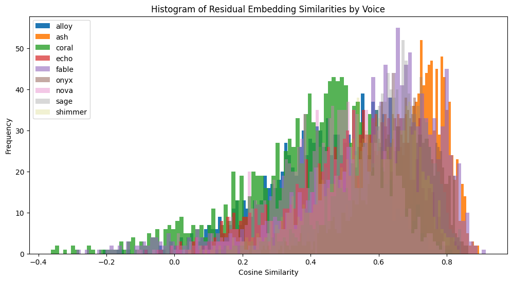
The histogram above displays the cosine similarity distributions of residual embeddings for each voice after regressing out the text content. Each colored distribution represents a specific voice (e.g., “alloy,” “ash,” “coral”), with the x-axis showing the cosine similarity values and the y-axis indicating the frequency of these values.
Key Observations:
Distinct Voice Distributions: The residual embeddings show noticeable differences in cosine similarity distributions for each voice, highlighting that voice-specific characteristics are preserved after text content is removed.
Cosine Similarity Range: Unlike the original audio embeddings, where cosine similarity values are tightly clustered due to shared text content, the residual embeddings exhibit a wider range of similarity values (from negative values to moderately high positives, up to ~0.8). This indicates reduced influence from shared text content.
To further illustrate the impact of residualization, we compare the similarity patterns of residual embeddings with those of the original audio embeddings. The next histogram visualizes the cosine similarity distributions of the original audio embeddings for each voice, offering a baseline to evaluate how much the shared text content influences these embeddings.
# Compute cosine similarity on the audio embeddings.
sim = cosine_similarity(df_audio_emb)
df_sim = pd.DataFrame(sim, index=df_audio_emb.index, columns=df_audio_emb.index)

# Plot histograms of the upper-triangle similarity values for each voice.
plt.figure(figsize=(12, 6))
alpha = 1.0  # starting alpha for histogram transparency

for voice in voices:
    # Select sample indices that contain the current voice.
    sample = [elem for elem in df_sim.index if voice in elem]
    mat = df_sim.loc[sample, sample]

    # Mask lower-triangle and diagonal values.
    mask = np.triu(np.ones(mat.shape, dtype=bool), k=1)
    upper_tri_values = np.where(mask, mat, np.nan).flatten()

    # Filter out NaN values.
    upper_tri_values = upper_tri_values[~np.isnan(upper_tri_values)]

    plt.hist(upper_tri_values, bins=100, label=voice, alpha=alpha)
    alpha -= 0.10

plt.legend()
plt.title("Histogram of Audio Embedding Similarities by Voice")
plt.xlabel("Cosine Similarity")
plt.ylabel("Frequency")
plt.show()
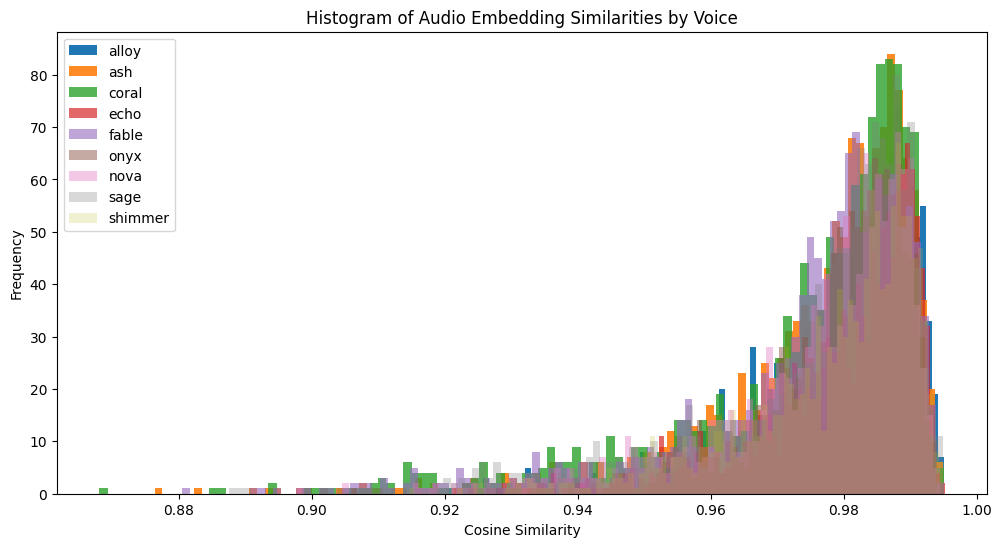
The histogram above displays the cosine similarity distributions for the original audio embeddings across different voices. Each colored distribution represents a specific voice (e.g., “alloy,” “ash,” “coral”), with the x-axis showing cosine similarity values and the y-axis indicating their frequency.
Key Observations:
Overlapping Voice Distributions: The similarity distributions for different voices overlap significantly, demonstrating that shared text content dominates the original audio embeddings.
High Similarity Concentration: The cosine similarity values for the original audio embeddings are tightly clustered in a high range, predominantly between 0.88 and 0.99, highlighting the strong influence of the text content.
Unlike the residual embeddings, the original audio embeddings exhibit a narrow spread of similarity values, indicating that speaker-specific features are less prominent in the original embeddings.
4.2 Same-Voice Similarity: Audio vs. Residual
In this section, we compare the cosine similarity patterns for recordings of the same voice (e.g., “alloy” vs. “alloy”) using both the original audio embeddings and the residual embeddings. The pairwise similarity matrices and histograms illustrate distinct differences between the two representations.
Original Audio Embeddings (Same Voice)
# Compute similarity for the same voice on audio embeddings.
voice_1 = "alloy"
voice_2 = "alloy"  # Same voice comparison.

sample_1 = [elem for elem in df_audio_emb.index if voice_1 in elem]
sample_2 = [elem for elem in df_audio_emb.index if voice_2 in elem]

pairwise_sim_same_audio = cosine_similarity(
    df_audio_emb.loc[sample_1],
    df_audio_emb.loc[sample_2]
)

plt.figure(figsize=(8, 6))
plt.pcolormesh(pairwise_sim_same_audio, cmap='viridis')
plt.title("Pairwise Similarity: 'alloy' vs. 'alloy' (Audio Embeddings)")
plt.colorbar()
plt.show()

plt.figure()
plt.hist(pairwise_sim_same_audio.flatten(), bins=100)
plt.title("Histogram: 'alloy' vs. 'alloy' (Audio Embeddings)")
plt.xlabel("Cosine Similarity")
plt.ylabel("Frequency")
plt.show()

print(pd.Series(pairwise_sim_same_audio.flatten()).describe())
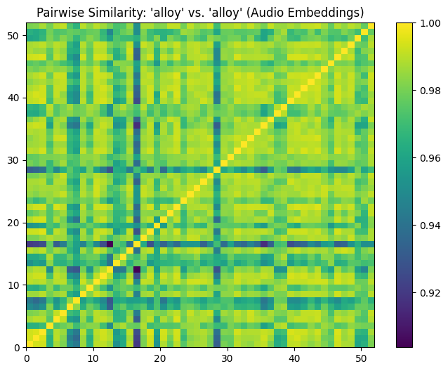
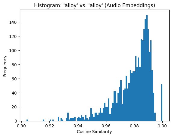
The similarity matrix for the original audio embeddings shows consistently high values, with most cosine similarity scores tightly clustered around 0.98. This is reflected in the histogram, where the majority of values fall between 0.95 and 1.0.
count    2704.000000
mean        0.978689
std         0.013633
min         0.903744
25%         0.972316
50%         0.982532
75%         0.988346
max         1.000000
dtype: float64
Residual Embeddings (Same Voice)
# Compute similarity for the same voice on residual embeddings.
sample_1_resid = [elem for elem in residual_emb.index if voice_1 in elem]
sample_2_resid = [elem for elem in residual_emb.index if voice_2 in elem]

pairwise_sim_same_resid = cosine_similarity(
    residual_emb.loc[sample_1_resid],
    residual_emb.loc[sample_2_resid]
)

plt.figure(figsize=(8, 6))
plt.pcolormesh(pairwise_sim_same_resid, cmap='viridis')
plt.title("Pairwise Similarity: 'alloy' vs. 'alloy' (Residual Embeddings)")
plt.colorbar()
plt.show()

plt.figure()
plt.hist(pairwise_sim_same_resid.flatten(), bins=100)
plt.title("Histogram: 'alloy' vs. 'alloy' (Residual Embeddings)")
plt.xlabel("Cosine Similarity")
plt.ylabel("Frequency")
plt.show()

print(pd.Series(pairwise_sim_same_resid.flatten()).describe())
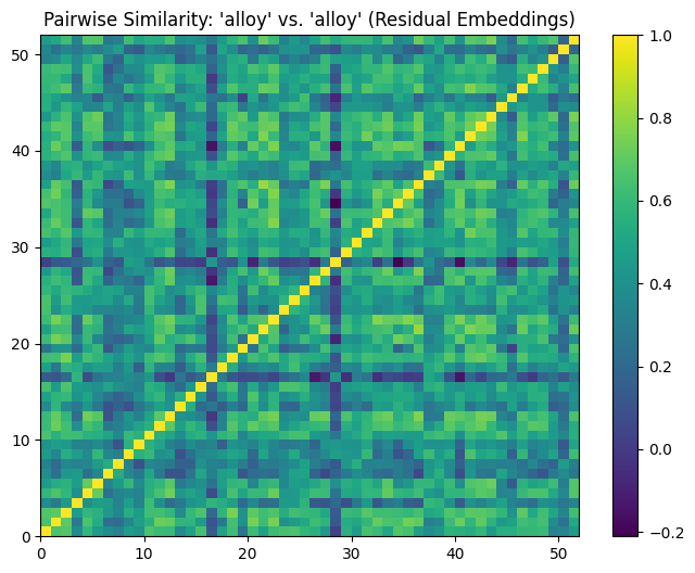
In contrast, the similarity matrix for the residual embeddings reveals a broader range of cosine similarity values, spanning from approximately -0.2 to 1.0. The histogram demonstrates more variability, with similarity values distributed more evenly across the range.
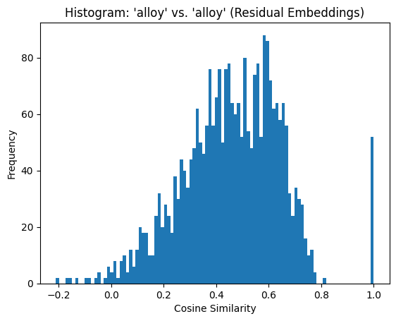
count    2704.000000
mean        0.460229
std         0.187644
min        -0.210560
25%         0.338727
50%         0.468087
75%         0.593228
max         1.000000
dtype: float64
4.3 Different-Voice Similarity: Audio vs. Residual
In this section, we analyze the similarity patterns for recordings of different voices (e.g., “alloy” vs. “coral”) using both the original audio embeddings and the residual embeddings.
The results provide insights into how shared text content and speaker-specific features influence embedding similarity.
Original Audio Embeddings (Different Voices)
# Compute similarity for different voices on audio embeddings.
voice_1 = "alloy"
voice_2 = "coral"  # different voice comparison.

sample_1 = [elem for elem in df_audio_emb.index if voice_1 in elem]
sample_2 = [elem for elem in df_audio_emb.index if voice_2 in elem]

pairwise_sim_same_audio = cosine_similarity(
    df_audio_emb.loc[sample_1],
    df_audio_emb.loc[sample_2]
)

plt.figure(figsize=(8, 6))
plt.pcolormesh(pairwise_sim_same_audio, cmap='viridis')
plt.title("Pairwise Similarity: 'alloy' vs. 'coral' (Audio Embeddings)")
plt.colorbar()
plt.show()

plt.figure()
plt.hist(pairwise_sim_same_audio.flatten(), bins=100)
plt.title("Histogram: 'alloy' vs. 'coral' (Audio Embeddings)")
plt.xlabel("Cosine Similarity")
plt.ylabel("Frequency")
plt.show()

print(pd.Series(pairwise_sim_same_audio.flatten()).describe())
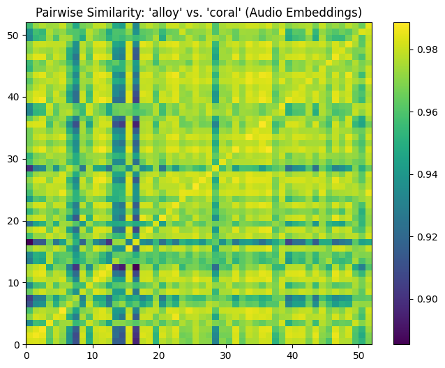
The similarity matrix and histogram for the original audio embeddings show that even for different voices, cosine similarity values remain high, with most scores clustering between 0.96 and 0.98. This indicates that shared text content dominates the embeddings, overwhelming the differences between voices. The high similarity values reflect a lack of discrimination between different speakers when text content is present.
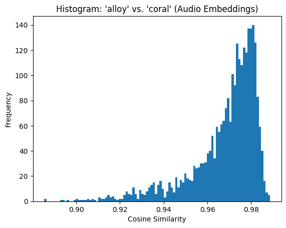
count    2704.000000
mean        0.968115
std         0.015492
min         0.885379
25%         0.962617
50%         0.972892
75%         0.978895
max         0.988612
dtype: float64
Residual Embeddings (Different Voices)
# Compute similarity for different voices on residual embeddings.
sample_1_resid = [elem for elem in residual_emb.index if voice_1 in elem]
sample_2_resid = [elem for elem in residual_emb.index if voice_2 in elem]

pairwise_sim_same_resid = cosine_similarity(
    residual_emb.loc[sample_1_resid],
    residual_emb.loc[sample_2_resid]
)

plt.figure(figsize=(8, 6))
plt.pcolormesh(pairwise_sim_same_resid, cmap='viridis')
plt.title("Pairwise Similarity: 'alloy' vs. 'coral' (Residual Embeddings)")
plt.colorbar()
plt.show()

plt.figure()
plt.hist(pairwise_sim_same_resid.flatten(), bins=100)
plt.title("Histogram: 'alloy' vs. 'coral' (Residual Embeddings)")
plt.xlabel("Cosine Similarity")
plt.ylabel("Frequency")
plt.show()

print(pd.Series(pairwise_sim_same_resid.flatten()).describe())
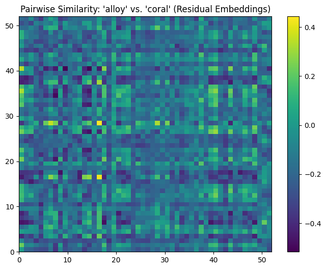
In stark contrast, the similarity matrix and histogram for the residual embeddings demonstrate a near-complete absence of similarity between different voices. The distribution of cosine similarity values spans a much wider range, centering around -0.15 with values as low as -0.5. This confirms that the residual embeddings have successfully removed the shared text content, leaving behind voice-specific characteristics. Since the embeddings now focus solely on speaker-related features, the similarity between different voices naturally drops.
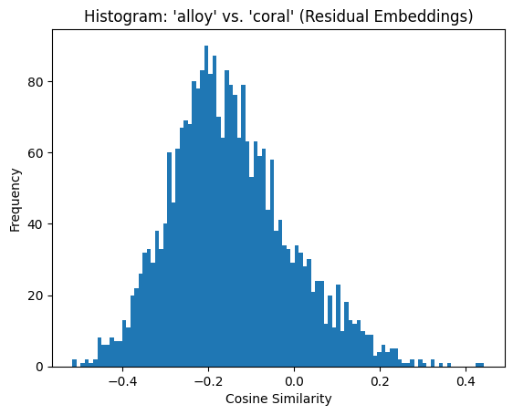
count    2704.000000
mean       -0.148577
std         0.139143
min        -0.516812
25%        -0.244333
50%        -0.161543
75%        -0.065892
max         0.443491
dtype: float64
The last histogram is particularly compelling, as it illustrates the impact of residualization by showing the near-complete absence of similarity between embeddings from different voices.
4.4 Average Similarity Across Voices
Finally, in this section, we compute the average pairwise cosine similarity between all combinations of voices for both the original and residual embeddings. This provides a broader summary of the effects observed in Sections 4.2 and 4.3 by generalizing the analysis to all voice pairs. Instead of examining the entire distribution of similarities, we condense the information into average values for each voice combination.
def plot_heatmap(sim_matrix, title, xtick_labels):
    plt.figure(figsize=(8, 6))
    plt.pcolormesh(sim_matrix, cmap='viridis')
    plt.title(title)
    plt.colorbar()
    tick_positions = np.arange(sim_matrix.shape[0]) + 0.5
    plt.xticks(tick_positions, xtick_labels, rotation=90)
    plt.yticks(tick_positions, xtick_labels)
    plt.show()

def compute_avg_similarity(df_emb, voices):
    n = len(voices)
    avg_sim = np.zeros((n, n))
    for i, v1 in enumerate(voices):
        for j, v2 in enumerate(voices):
            sample_1 = [elem for elem in df_emb.index if v1 in elem]
            sample_2 = [elem for elem in df_emb.index if v2 in elem]
            sim_vals = cosine_similarity(df_emb.loc[sample_1], df_emb.loc[sample_2])
            avg_sim[i, j] = np.nanmean(sim_vals.flatten())
    return avg_sim

# Average similarity on audio embeddings.
sim_audio = compute_avg_similarity(df_audio_emb, voices)
plot_heatmap(sim_audio,
             "Average Similarity Between Voices (Audio Embeddings)",
             voices)

# Average similarity on residual embeddings.
sim_resid = compute_avg_similarity(residual_emb, voices)
plot_heatmap(sim_resid,
             "Average Similarity Between Voices (Residual Embeddings)",
             voices)
Original Audio Embeddings
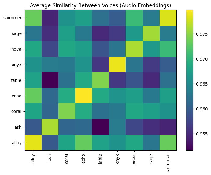
The heatmap of average pairwise similarities for the original audio embeddings reveals uniformly high similarity values across all voice pairs, with most values exceeding 0.96. This aligns with the earlier observations that text content dominates the original embeddings. The lack of variability in the heatmap suggests that the original embeddings do not effectively distinguish between voices, as the textual content contributes significantly to the similarity scores.
Residual Embeddings
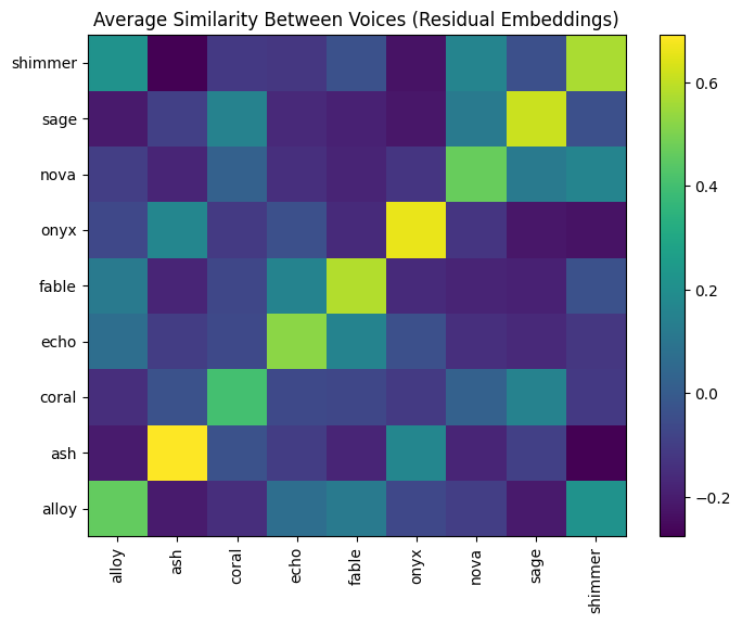
In contrast, the heatmap for the residual embeddings shows low or negative similarity values for different voice pairs, illustrating the success of residualization in removing text content. For the same voice combinations (diagonal elements of the heatmap), the values are noticeably higher, reflecting the preservation of speaker-specific features. The strong contrast between diagonal and off-diagonal values demonstrates that the residual embeddings capture meaningful differences between voices while retaining consistency within the same voice.
5. Discussion and Conclusion
Our analysis shows that the original audio embeddings exhibit high similarity across different voices, likely due to the dominating influence of text content (since all voices speak the same sentence). After applying Ridge regression to regress out the text component, the residual embeddings show:
- High within-voice similarity: The residual still captures speaker-specific characteristics.
- Low between-voice similarity: The shared text content is largely removed.
In this blog, we demonstrated how regression can effectively isolate speaker-specific features in audio embeddings by removing shared text content. However, we did not analyze in depth what characteristics remain in the residual embeddings. Do they capture pitch, tone, prosody, timbre, speaking rate, vocal intensity, or background noise? These are open questions worth further exploration. In future posts, we aim to explore these residual features in greater detail, shedding light on the nuances of what these embeddings truly represent and how they can be applied to more specialized audio analysis tasks.