Speaker identification in 'Marine Le Pen vs. Emmanuel Macron 2017 French Presidential Debate'

Speaker identification in ‘Marine Le Pen vs. Emmanuel Macron 2017 French Presidential Debate’
Only a couple of days before the 2022 live televised presidential debate between Marine Le Pen and President Emmanuel Macron, I took the time to download historical presidential election debates from the first one in 1974 to these days (thanks Benjamin H. and his friend for the audio recordings) for basic speech signal analysis.
While working on these recordings, I noticed that form and content changed a lot over the past 50 years, and not for the better…
In this blog, I just illustrate the task of speaker identification: Who is speaking, and when?
This can be done relatively well with basic Machine Learning tools (Gaussian Mixture Models).
One could also try to do better by adding a Hidden Markov Model (HMM) on top, or using a deep learning approach such as LSTM or 1D ConvNet.
As usual with ‘real life’ projects, one starts without any labels for learning supervision.
import pydub
import numpy as np
import pandas as pd
from tqdm import tqdm
import sounddevice as sd
from sklearn import preprocessing
from sklearn.mixture import GaussianMixture
import python_speech_features as mfcc
import matplotlib.pyplot as plt
Loading the data
Some piece of code to read a mp3 file into a numpy array:
def read(f, normalized=False):
    """MP3 to numpy array"""
    a = pydub.AudioSegment.from_mp3(f)
    y = np.array(a.get_array_of_samples())
    if a.channels == 2:
        y = y.reshape((-1, 2))
    if normalized:
        return a.frame_rate, np.float32(y) / 2**15
    else:
        return a.frame_rate, y

def write(f, sr, x, normalized=False):
    """numpy array to MP3"""
    channels = 2 if (x.ndim == 2 and x.shape[1] == 2) else 1
    if normalized:
        y = np.int16(x * 2 ** 15)
    else:
        y = np.int16(x)
    song = pydub.AudioSegment(
        y.tobytes(), frame_rate=sr,
        sample_width=2, channels=channels)
    song.export(f, format="mp3", bitrate="320k")
The code below is used to extract Mel Frequency Cepstral Coefficient (MFCC).
The feature space consists in these coefficients, and the temporal deltas of these coefficients.
These features are known to be very effective for automatic speech recognition.
The MFCC features can be easily computed using the python_speech_features library.
def calculate_delta(array):
    rows, cols = array.shape
    deltas = np.zeros((rows, 20))
    N = 2
    for i in range(rows):
        index = []
        j = 1
        while j <= N:
            if i - j < 0:
                first = 0
            else:
                first = i - j
            if i + j > rows - 1:
                second = rows - 1
            else:
                second = i + j
            index.append((second, first))
            j += 1
        deltas[i] = (array[index[0][0]] -
                     array[index[0][1]] +
                     (2 * (array[index[1][0]] -
                           array[index[1][1]]))) / 10
    return deltas


def extract_features(audio, rate):
    mfcc_feature = mfcc.mfcc(
        audio,rate, 0.025, 0.01, 20,
        nfft=1200, appendEnergy=True)
    mfcc_feature = preprocessing.scale(mfcc_feature)
    delta = calculate_delta(mfcc_feature)
    combined = np.hstack((mfcc_feature, delta))
    return combined
We read the whole debate into a numpy array:
%%time

sampling_rate, audio = read(
    'debats/2017 - Marine Le Pen - Emmanuel Macron.mp3')
CPU times: user 1.42 s, sys: 1.87 s, total: 3.29 s
Wall time: 9.08 s
The audio signal is sampled at 44 kHz:
sampling_rate
44100
The debate has a duration around 2h40:
audio.shape[0] / sampling_rate / 3600
2.5995255228017133
If you want to listen to the whole debate in your notebook:
import IPython

IPython.display.Audio(
    "debats/2017 - Marine Le Pen - Emmanuel Macron.mp3")
Bootstrapping initial labels
As with most ‘original’ work, one starts without any labels. We will take some time to find sections of the audio recording where there is a clearly identified speaker.
The universe of ‘speakers’ is:
{
    'Marine Le Pen',
    'Emmanuel Macron',
    'Christophe Jakubyszyn',
    'Nathalie Saint-Cricq',
    'jingle',
}
samples = {
    'Marine Le Pen': audio[7_700_000:13_160_000],
    'Emmanuel Macron': np.vstack(
        (audio[13_350_000:18_610_000],
         audio[18_850_000:19_560_000])),
    'Christophe Jakubyszyn': np.vstack(
        (audio[5_360_000: 6_040_000],
         audio[6_330_000: 6_775_000],
         audio[7_050_000: 7_700_000])),
    'Nathalie Saint-Cricq': np.vstack(
        (audio[6_040_000: 6_330_000],
         audio[6_780_000: 7_010_000],
         audio[19_560_000: 20_460_000])),
    'jingle': np.vstack(
        (audio[:400_000],
         audio[-800_000:])),
}
gmm_models = {}
for name, sample in samples.items():
    features = extract_features(sample, sampling_rate)
    gmm = GaussianMixture(n_components=10,
                          max_iter=500,
                          covariance_type='diag',
                          n_init=10)
    gmm.fit(features)
    gmm_models[name] = gmm
Testing the GMMs on a random (out)sample
outsample = audio[312_700_000:312_900_000]
sd.play(outsample, sampling_rate)
This is obviously Emmanuel Macron speaking for 4.5 seconds:
(312_900_000 - 312_700_000) / sampling_rate
4.535147392290249
features = extract_features(outsample, sampling_rate)
scores = sorted(
    [(round(gmm.score(features), 2), name)
     for name, gmm in gmm_models.items()],
    key=lambda x: x[0],
    reverse=True)
scores
[(-21.18, 'Emmanuel Macron'),
 (-22.34, 'Christophe Jakubyszyn'),
 (-24.22, 'Marine Le Pen'),
 (-24.52, 'Nathalie Saint-Cricq'),
 (-28.94, 'jingle')]
Given this short audio sample, it is the Gaussian Mixture Model associated to Emmanuel Macron which has the highest log-likehood.
Since all the five Gaussian Mixture Models have the same number of parameters, we can conclude that the Gaussian Mixture Model associated to Emmanuel Macron represents the data the best, and thus Emmanuel Macron is the speaker in this audio sample (which is correct).
Note that the second best model is the one for Christophe Jakubyszyn (a man – journalist), then Marine Le Pen (a woman) who has a deeper voice than Nathalie Saint-Cricq (another woman – journalist). Finally, the model associated with jingles (very distinct from speech) is by far the worst.
Definition of a simple classifier
We define the following classifier which finds the most likely speaker based on the log-likelihood of its associated GMM model:
def classifier(models, features):
    scores = [gmm.score(features) for gmm in models.values()]
    return np.argmax(scores)
Running the classifier on the previous (out)sample gives:
list(gmm_models.keys())[classifier(gmm_models, features)]
'Emmanuel Macron'
A first pass at labelling the debate
STEP = 200_000
starts = [i * STEP for i in range(len(audio) // STEP)]
labels = np.zeros(len(audio))
for start in tqdm(starts):
    f = extract_features(
            audio[start:start + STEP], sampling_rate)
    labels[start:start + STEP] = classifier(gmm_models, f)
100%|███████████████████████████████████████| 2063/2063 [01:05<00:00, 31.48it/s]
We can quickly check the speaking time of the different people:
for i in range(len(gmm_models)):
    print(labels[labels == i].shape[0],
          list(gmm_models.keys())[i])
197100672 Marine Le Pen
174200000 Emmanuel Macron
20600000 Christophe Jakubyszyn
19400000 Nathalie Saint-Cricq
1400000 jingle
We note that the presidential candidates talk roughly 10 times more than the journalists. Roughly same time for both candidates, and for both journalists.
A second pass at labelling the debate
Now that all the audio recording has been labelled sample by sample with an identified speaker, we can fit the GMMs again over the whole dataset. In some cases, with much more labeled data points, it can help improve the initial classification.
samples = {
    'Marine Le Pen': audio[labels == 0],
    'Emmanuel Macron': audio[labels == 1],
    'Christophe Jakubyszyn': audio[labels == 2],
    'Nathalie Saint-Cricq': audio[labels == 3],
    'jingle': audio[labels == 4],
}

gmm_models = {}
for name, sample in tqdm(samples.items()):
    features = extract_features(sample, sampling_rate)
    gmm = GaussianMixture(n_components=10,
                          max_iter=500,
                          covariance_type='diag',
                          n_init=10)
    gmm.fit(features)
    gmm_models[name] = gmm
100%|████████████████████████████████████████████| 5/5 [11:14<00:00, 134.88s/it]
for i in range(len(gmm_models)):
    print(labels[labels == i].shape[0],
          list(gmm_models.keys())[i])
197100672 Marine Le Pen
174200000 Emmanuel Macron
20600000 Christophe Jakubyszyn
19400000 Nathalie Saint-Cricq
1400000 jingle
It seems that we have already reached a fixed point: The classification did not change.
Speaking time and distribution of talk durations
Provided the classification is close to perfect, we can study some basic features such as for how long they speak in total (supposed to be exactly the same as per the debate rules), and how long when it is their turn to speak. Note that this particular debate was full of interruptions (unlike the 1974 one which was very orderly, for example).
Speaking time
_labels = pd.Series(labels)
speakers = _labels.loc[starts]
names = list(gmm_models.keys())
for i in range(len(gmm_models)):
    speakers = speakers.replace(i, names[i])
speakers.value_counts()
Marine Le Pen            985
Emmanuel Macron          871
Christophe Jakubyszyn    103
Nathalie Saint-Cricq      97
jingle                     7
dtype: int64
Converting back the samples length to minutes:
speakers.value_counts() * (STEP / sampling_rate) / 60
Marine Le Pen            74.452003
Emmanuel Macron          65.835223
Christophe Jakubyszyn     7.785336
Nathalie Saint-Cricq      7.331822
jingle                    0.529101
dtype: float64
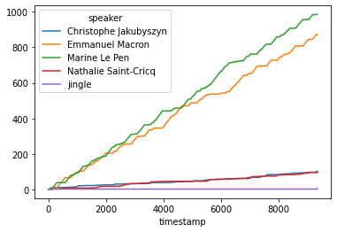
Note that there is a discrepancy of 10 minutes between the two candidates! which should not be possible. It may come from misclassification from the model, but most likely due to the times where Marine Le Pen impolitely interrupted and interjected during Emmanuel Macron answers. This time may not have been measured appropriately by the debate organizers… To be investigated further: I do not know the exact rules for attributing speaking time to one or the other. Note that many times both were trying to outloud the other candidate.
_speakers = speakers.reset_index()
_speakers['v'] = 1
_speakers.columns = ['timestamp', 'speaker', 'v']
_speakers['timestamp'] = _speakers['timestamp'] / sampling_rate
is_talking = _speakers.pivot(
    index='timestamp', columns='speaker', values='v')
is_talking.cumsum().fillna(method='ffill').plot();

Note that the difference in speaking time between the two candidates built up during the second half of the debate.
Distribution of talk durations
def compute_speech_durations(is_talking, name):
    _tmp = is_talking.reset_index(drop=True)
    cls_chunks = _tmp[name].dropna().index.values
    talk_durations = []
    count = 1
    for i in range(len(cls_chunks) - 1):
        if cls_chunks[i] + 1 == cls_chunks[i + 1]:
            count += 1
        else:
            talk_durations.append(count * STEP / sampling_rate)
            count = 1
    return pd.Series(talk_durations)
for name in ['Emmanuel Macron', 'Marine Le Pen']:
    talk_durations = compute_speech_durations(is_talking, name)
    plt.hist(talk_durations,
             density=True,
             bins=20,
             log=True,
             label=name,
             alpha=0.6)
plt.legend()
plt.show()

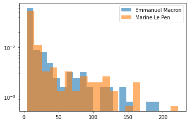
There is no clear pattern in the distribution of the uninterrupted talk durations. The longest bit is below 4 minutes.
for name in ['Christophe Jakubyszyn', 'Nathalie Saint-Cricq']:
    talk_durations = compute_speech_durations(is_talking, name)
    plt.hist(talk_durations,
             density=True,
             bins=10,
             log=True,
             label=name,
             alpha=0.6)
plt.legend()
plt.show()

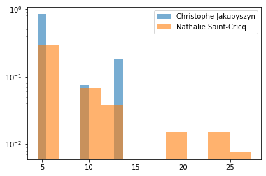
Journalists in this debate don’t say much except trying to balance talking time between the two candidates, and forcing them to progress along predefined broad topics. The speaking time between the two journalists is very similar.
What’s next?
In this short blog post, we did an elementary processing of the 2017 presidential debate audio recording, namely speaker identification. This is a first step before more advanced tasks.
What can we do next?
I am no political scientist, but things that might be of interest to study in the audio recordings (information not readily available in transcripts) are:
- evolution of the speaking time and distributions patterns (compare to previous debates since 1974)
- constant tone through the debate or major changes?
- quantify aggressivity in answers
- measure the tendency to interrupt the other candidate, evolution through time during the debate, and previous ones
- how much hesitation in answers
- measure differences to a baseline when previous debates are available (relatively easy to research)
- lies detection (any particular audio cues? specific to the candidate?) – needs a knowledge base to identify false claims: not trivial!