Ellipsoids covariance matrices A few ellipsoids representing the associated covariance matrices along the geodesic path from the leftmost to the rightmost matrices.

The Swelling Effect: Think twice before averaging covariance matrices

Covariance (and correlation) matrices are ubiquitous in science, and quantitative finance. They are known to be hard to estimate, and more often than not practitioners apply various geometric operations (e.g. averaging, shrinkage) and projections (e.g. Higham’s) using Frobenius norm (the standard Euclidean norm, and induced distance, on matrices) without thinking too much about the implications of this particular geometry.

In this blog, we illustrate the swelling effect which is an artifact of applying Euclidean geometry on the space of SPD matrices.

For finance practitioners, this means that you artificially inflate the determinant of your system, which practically translates to a) seeing more diversification potential than there really is; and/or b) seeing more variance in certain eigen-directions than there really is.

import numpy as np
from scipy.linalg import (
    expm, logm, sqrtm, fractional_matrix_power)
import matplotlib.pyplot as plt
from matplotlib.patches import Ellipse

Let’s consider the space of SPD matrices of fixed dimension $m \geq 2$ denoted by $\mathcal{S_m^+}$.

Any matrix $S \in \mathcal{S_m^+}$ can be written $S = LL^\top$ with $L$ a lower triangular matrix whose diagonal elements are positive (Cholesky decomposition). The space of lower triangular matrices with positive diagonal with dimension $m \geq 2$ is denoted $\mathcal{L}_m^+$. When $S \in \mathcal{S_m^+}$, the Cholesky decomposition $S = LL^\top$, with $L \in \mathcal{L}_m^+$, is unique.

Notations:

$\| \cdot \|_F$ is the Frobenius norm, i.e. $\| M \|_F = \sqrt{\sum_{i,j} m_{ij}^2}$ for $M \in \mathcal{M}_m(\mathbb{R})$ .

$\lfloor M \rfloor$ is the strict lower triangular part of matrix $M \in \mathcal{M}_m(\mathbb{R})$ (i.e. zero diagonal and zero upper triangular)

$\mathbb{D}(M)$ is the diagonal of matrix $M \in \mathcal{M}_m(\mathbb{R})$ (i.e. strict lower and upper triangular are zero).

Swelling effect: The determinant of the average is larger than any of the original determinants.

The Euclidean average of SPD matrices suffers from the swelling effect.

Numerical experiments:

Let $S_1 = \begin{pmatrix} 3 & 1 \\ 1 & 2 \end{pmatrix}$ and $S_2 = \begin{pmatrix} 6 & 5 \\ 5 & 5 \end{pmatrix}.$ Note that $\det(S_1) = \det(S_2) = 5$.

We will display a few covariance matrices along the geodesic path between $S_1$ and $S_2$ for several SPD metrics: Euclidean, Cholesky, Riemannian Affine-Invariant, Riemannian Log-Euclidean, Riemannian Log-Cholesky. We will also track their determinant to see whether they are affected by swelling.

S1 = np.array([[3, 1], [1, 2]])
eigenvals_1, eigenvecs_1 = np.linalg.eig(S1)
idx = np.argsort(eigenvals_1)[::-1]
eigenvals_1 = eigenvals_1[idx]
eigenvecs_1 = eigenvecs_1[:, idx]

S2 = np.array([[6, 5], [5, 5]])
eigenvals_2, eigenvecs_2 = np.linalg.eig(S2)
idx = np.argsort(eigenvals_2)[::-1]
eigenvals_2 = eigenvals_2[idx]
eigenvecs_2 = eigenvecs_2[:, idx]

Below, a plotting function to illustrate how the SPD matrix and its determinant evolve along the geodesic between $S_1$ and $S_2$.

# plotting function
def plot_geodesic(S1, S2, geod):
    fig, ax = plt.subplots(figsize=(16, 16), subplot_kw={'aspect': 'equal'})
    nb_steps = 10
    dets = []
    for t in np.linspace(0, 1, nb_steps):
        St = geod(S1, S2, t)
        eigenvals, eigenvecs = np.linalg.eig(St)
        idx = np.argsort(eigenvals)[::-1]
        eigenvals = eigenvals[idx]
        eigenvecs = eigenvecs[:, idx]

        dets.append(np.prod(eigenvals))

        vec1 = eigenvals[0] * eigenvecs[:, 0]
        vec2 = eigenvals[1] * eigenvecs[:, 1]
        angle = np.arccos(np.dot(eigenvecs[:, 0], [1, 0])) * 180 / np.pi

        shift = 40 * t    

        plt.plot([shift + 0, shift + vec1[0]], [0, vec1[1]],
                 color='blue')
        plt.plot([shift + 0, shift + vec2[0]], [0, vec2[1]],
                 color='blue')

        ellipse = Ellipse((shift, 0),
                          width=eigenvals[0] * 2,
                          height=eigenvals[1] * 2,
                          angle=angle)

        ax.add_artist(ellipse)
        ellipse.set_alpha(0.2)

    ax.set_xlim(-4, 48)
    ax.set_ylim(-8, 8)
    plt.title('Ellipsoids representing $2 \\times 2$ SPD matrices ' +
              'along the geodesic path from $S_1$ to $S_2$',
              fontsize=20)
    plt.show()


    plt.figure(figsize=(16, 6))
    plt.plot(dets)
    plt.title('Determinants along the geodesic path from $S_1$ to $S_2$',
              fontsize=20)
    plt.show()

Euclidean metric

distance

$S_1, S_2 \in \mathcal{S_m^+}$,

$d_{eucl}(S_1, S_2) = \| S_1 - S_2 \|_F$

geodesic

$\gamma : t \in [0, 1] \rightarrow (1 - t) S_1 + t S_2$

Frechet mean

$S_1, \ldots, S_n \in \mathcal{S_m^+}$,

$\text{argmin}_{S \in \mathcal{S_m^+}} \sum_{i=1}^n d_{eucl}(S, S_i)^2 = \frac{1}{n} \sum_{i=1}^n S_i$

def euclidean_geodesic(S1, S2, t):
    return (1 - t) * S1 + t * S2

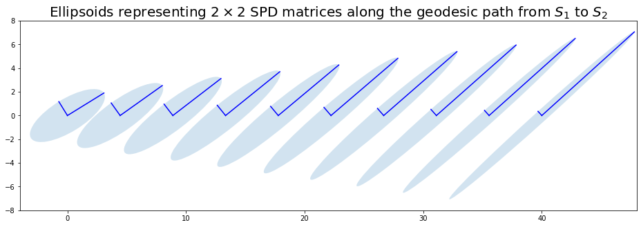
plot_geodesic(S1, S2, euclidean_geodesic)

Ellipsoids covariance matrices

Full swelling effect

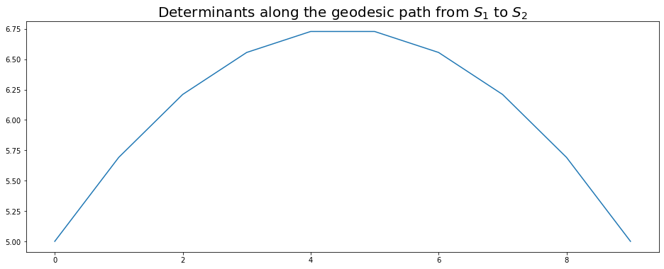
Very noticeable swelling effect!

Cholesky metric

distance

$S_1, S_2 \in \mathcal{S_m^+}$, $S_1 = L_1 L_1^\top$, $S_2 = L_2 L_2^\top$,

$d_{chol}(S_1, S_2) = \|L_1 - L_2\|_F$

geodesic

$\gamma : t \in [0, 1] \rightarrow \left((1 - t) L_1 + t L_2\right) \left((1 - t) L_1 + t L_2\right)^\top$

Frechet mean

$S_1, \ldots, S_n \in \mathcal{S_m^+}$,

$\text{argmin}_{S \in \mathcal{S_m^+}} \sum_{i=1}^n d_{chol}(S, S_i)^2 = \left(\frac{1}{n} \sum_{i=1}^n L_i\right) \left(\frac{1}{n} \sum_{i=1}^n L_i\right)^\top$

def cholesky_geodesic(S1, S2, t):
    L1 = np.linalg.cholesky(S1)
    L2 = np.linalg.cholesky(S2)
    return ((1 - t) * L1 + t * L2).dot(((1 - t) * L1 + t * L2).T)

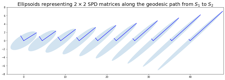
plot_geodesic(S1, S2, cholesky_geodesic)

Ellipsoids covariance matrices

Full swelling effect

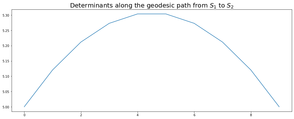
The Cholesky distance also suffers from the swelling effect, but it is less severe than the Euclidean case.

Riemannian Affine-Invariant metric

– no closed form found so far for the Frechet average of SPD matrices

++ closed form for parallel transport along geodesics

++ easy-to-compute exponential and logarithmic maps

distance

$d_{airm}(S_1, S_2) = \|\log(S_1^{-1} S_2)\|_F = \left(\sum_{i=1}^m \log^2 \lambda_i\right)^{1/2}$

where the $\lambda_i$ are the strictly positive eigenvalues of $S_1^{-1} S_2$.

geodesic

$\gamma : t \in [0, 1] \rightarrow S_1^{1/2} \left(S_1^{-1/2} S_2 S_1^{-1/2}\right)^t S_1^{1/2}$

Frechet mean

No known closed formula. The Frechet mean can be computed using a gradient descent algorithm (cf. Intrinsic Statistics on Riemannian Manifolds: Basic Tools for Geometric Measurements).

def airm_geodesic(S1, S2, t):
    sqrt_S1 = sqrtm(S1)
    inv_sqrt_S1 = np.linalg.inv(sqrt_S1)
    m = inv_sqrt_S1.dot(S2.dot(inv_sqrt_S1))
    e = fractional_matrix_power(m, t)
    return sqrt_S1.dot(e.dot(sqrt_S1))

plot_geodesic(S1, S2, airm_geodesic)

Ellipsoids covariance matrices

Full swelling effect

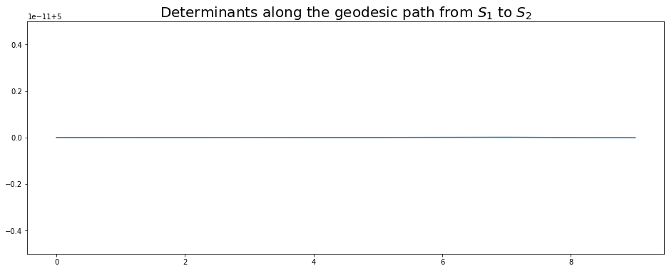
No swelling effect.

Riemannian Log-Euclidean metric

++ closed form of the Frechet average of SPD matrices

– computation of Riemannian exponential and logarithmic maps requires evaluating a series of an infinite number of terms

distance

$S_1, S_2 \in \mathcal{S_m^+}$,

$d_{loge}(S_1, S_2) = \| \log S_2 - \log S_1 \|_F$

geodesic

$\gamma : t \in [0, 1] \rightarrow \exp\left((1-t) \log S_1 + t \log S_2 \right)$

Frechet mean

$S_1, \ldots, S_n \in \mathcal{S_m^+}$,

$\text{argmin}_{S \in \mathcal{S_m^+}} \sum_{i=1}^n d_{eucl}(S, S_i)^2 = \exp\left(\frac{1}{n} \sum_{i=1}^n \log S_i\right)$

def log_euclidean_geodesic(S1, S2, t):
    return expm((1 - t) * logm(S1) + t * logm(S2))

plot_geodesic(S1, S2, log_euclidean_geodesic)

Ellipsoids covariance matrices

Full swelling effect

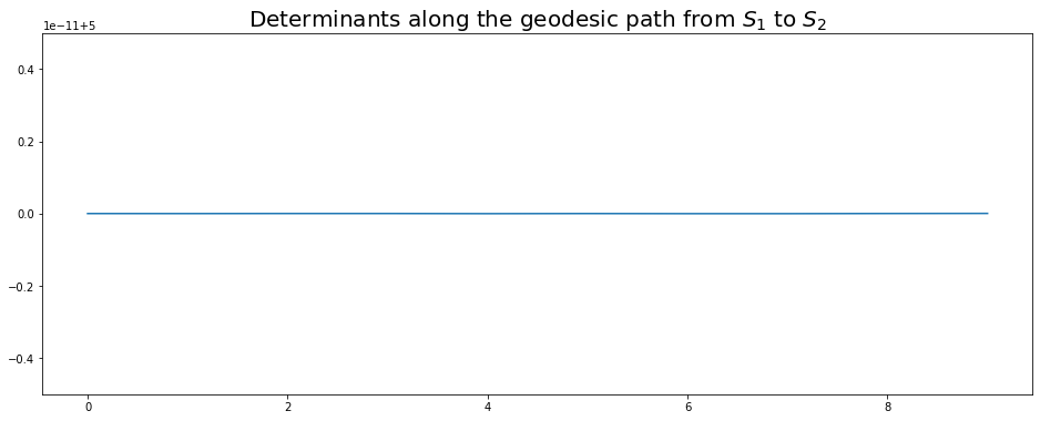
No swelling effect.

Riemannian Log-Cholesky metric

++ closed form for the Log-Cholesky average of SPD matrices

++ simple and easy-to-compute expressions for Riemannian exponential and logarithmic maps

++ simple and easy-to-compute expression for parallel transport along geodesics

distance

$S_1 = L_1 L_1^\top$, $S_2 = L_2 L_2^\top$,

$d_{logc}(S_1, S_2) = \left( \| \lfloor L_1 \rfloor - \lfloor L_2 \rfloor \|_F^2 + \|\log \mathbb{D}(L_1) - \log \mathbb{D}(L_2) \|_F^2 \right)^{1/2}$

geodesic

$\gamma_{logc} : t \in [0, 1] \rightarrow \lfloor L_1 \rfloor + t (\lfloor L_2 \rfloor - \lfloor L_1 \rfloor) + \mathbb{D}(L_1) \exp\left(t \left(\log \mathbb{D}(L_2) - \log \mathbb{D}(L_1) \right)\right)$

$\gamma : t \in [0, 1] \rightarrow \gamma_{logc}(t) \gamma_{logc}(t)^\top$

Frechet mean

$S_1, \ldots, S_n \in \mathcal{S_m^+}$,

$\text{argmin}_{S \in \mathcal{S_m^+}} \sum_{i=1}^n d_{logc}(S, S_i)^2 = \left(\frac{1}{n} \sum_{i=1}^n \lfloor L_i \rfloor + \exp \left( \frac{1}{n} \sum_{i=1}^n \log \mathbb{D}(L_i) \right) \right) \left(\frac{1}{n} \sum_{i=1}^n \lfloor L_i \rfloor + \exp \left( \frac{1}{n} \sum_{i=1}^n \log \mathbb{D}(L_i) \right) \right)^\top$

def log_cholesky_geodesic(S1, S2, t):
    idx = np.triu_indices_from(S1, k=0)
    L1 = np.linalg.cholesky(S1)
    L2 = np.linalg.cholesky(S2)
    tril_L1 = L1.copy()
    tril_L2 = L2.copy()
    tril_L1[idx] = 0
    tril_L2[idx] = 0
    diag_L1 = np.diag(np.diag(L1))
    diag_L2 = np.diag(np.diag(L2))
    log_chol_geod = tril_L1 + t * (tril_L2 - tril_L1) + diag_L1.dot(
        expm(t * (logm(diag_L2) - logm(diag_L1))))
    return log_chol_geod.dot(log_chol_geod.T)

plot_geodesic(S1, S2, log_cholesky_geodesic)

Ellipsoids covariance matrices

Full swelling effect

No swelling effect.

Conclusion: One has to be aware of this effect when doing moving average of covariance matrices, shrinkage, Higham Euclidean projections in quantitative finance…