Bayesian Networks for Business: Modeling Profit and Loss of a Cafe in Hong Kong
Bayesian Networks for Business: Modeling Profit and Loss of a Cafe in Hong Kong
Why Do Tai Hang’s Coffee Shops Keep Failing?
tl;dr Decreasing foot traffic, driven by a significant decline in the western expatriate population.
Context: The once vibrant Tai Hang neighborhood has seen a notable drop in its rich western population, as both anecdotal evidence, and to some extent our paper Mapping Hong Kong’s Financial Ecosystem studying the Hong Kong SFC public register demographics, suggest. This shift has heavily impacted local businesses, particularly coffee shops, struggling to attract enough patrons to stay afloat.
The bustling neighborhoods of Tin Hau and Tai Hang in Hong Kong have long been hotspots for coffee enthusiasts, drawing in strong foot traffic and Instagram influencers eager to capture the next aesthetic moment. However, since the COVID-19 pandemic, these once-thriving coffee shops have faced a significant decline. Despite beautifully designed interiors and quality coffee—often accompanied by excellent food—many of these businesses don’t last more than a year or two. It’s a perplexing trend, with new cafes continually popping up, only to close down shortly after. Why are so many coffee shops failing, and yet people keep trying their hand at running them?
This brings us to a key question: What does it take to break even in the cafe business? Can we estimate how much profit, or loss, a typical coffee shop would make in a year? How much risk is involved, and is it worth the effort to operate such a business?
In this blog, we’ll explore these questions by building a simple Bayesian network model to simulate the profit-and-loss (P&L) of a coffee shop over the course of a year. We’ll focus on key variables—like daily foot traffic, average bill size, rent, wages, and raw material costs—without diving into the complexities of setup costs (such as renovation, licenses, and administrative expenses). By simulating daily P&L across different scenarios, we aim to gain insights into the financial realities of running a cafe.
Although our model will remain simple for now, avoiding factors like customer reviews, seasonality, competition, and broader economic conditions, it provides a useful starting point. We also plan to gather feedback from F&B industry experts to validate whether our base assumptions align with current market conditions.
Ultimately, the simulations will show that operating a cafe is no easy feat, with potential annual P&L ranging between -3 million HKD and 2 million HKD. This blog will offer a clear view into the financial rollercoaster that is running a coffee shop in today’s Hong Kong.
import numpy as np
import pandas as pd
import networkx as nx
from tqdm import tqdm
import matplotlib.pyplot as plt

from pgmpy.factors.continuous import LinearGaussianCPD
from pgmpy.models import LinearGaussianBayesianNetwork
In this blog post, we will use pgmpy, a Bayesian networks library.
Using pgmpy, we will define continuous Conditional Probability Distributions (CPDs) and model the key relationships between variables that drive the profit-and-loss dynamics of a cafe. This will enable us to simulate and better understand the financial outcomes of running a coffee shop under different conditions.
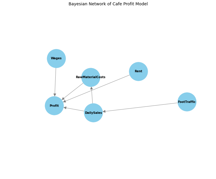
In our model, we define key variables that influence the daily profit of a coffee shop. The number of daily visitors, or FootTraffic, directly impacts DailySales, as more patrons generally translate to higher revenue. DailySales, in turn, affects two key cost drivers: RawMaterialCosts (the expense of ingredients and consumables) and Profit. The higher the sales, the more materials are needed, increasing costs. Additionally, Wages (fixed costs for staff) and Rent (fixed operating costs) both influence the Profit. By linking these variables, we model how changes in foot traffic, sales, and costs affect the cafe’s profitability on a daily basis.
We define the model in the cell below:
def build_model(average_bill=60, average_traffic=100, daily_rent=2000, daily_wage=1200):

    model = LinearGaussianBayesianNetwork([
        ('FootTraffic', 'DailySales'),
        ('DailySales', 'RawMaterialCosts'),
        ('DailySales', 'Profit'),
        ('RawMaterialCosts', 'Profit'),
        ('Wages', 'Profit'),
        ('Rent', 'Profit'),
    ])

    # Define the CPD for FootTraffic (independent variable)
    cpd_foot_traffic = LinearGaussianCPD('FootTraffic', [average_traffic], (0.1 * average_traffic)**2)

    # Define the CPD for DailySales as a function of FootTraffic
    cpd_daily_sales = LinearGaussianCPD(
        'DailySales',
        [0, average_bill],
        (0.1 * average_bill)**2,
        ['FootTraffic']
    )

    # Define the CPD for RawMaterialCosts as a function of DailySales
    cpd_raw_material_costs = LinearGaussianCPD('RawMaterialCosts', [100, 0.4], 20, ['DailySales'])

    cpd_wages = LinearGaussianCPD('Wages', [daily_wage], 0)  # Fixed cost for wages

    cpd_rent = LinearGaussianCPD('Rent', [daily_rent], 0)  # Fixed cost for rent

    # Define the CPD for Profit as a function of DailySales, RawMaterialCosts, Wages, and Rent
    cpd_profit = LinearGaussianCPD(
        'Profit', [0, 1, -1, -1, -1], 10, ['DailySales', 'RawMaterialCosts', 'Wages', 'Rent'])

    # Add CPDs to the model
    model.add_cpds(
        cpd_foot_traffic,
        cpd_daily_sales,
        cpd_raw_material_costs,
        cpd_wages,
        cpd_rent,
        cpd_profit
    )

    assert model.check_model()

    return model
In the cell above, we build a Bayesian network model that simulates the daily profit of a coffee shop based on several variables: FootTraffic, DailySales, RawMaterialCosts, Wages, Rent, and Profit. Let’s break down the model and the logic behind it.
Network Structure:
The model connects the variables as follows:
-
FootTraffic → DailySales: The number of people visiting the cafe directly affects the daily sales. We use FootTraffic as an input variable to predict DailySales.
-
DailySales → RawMaterialCosts & Profit: The sales determine the raw material costs (since higher sales require more ingredients) and also directly contribute to profit.
-
RawMaterialCosts, Wages, Rent → Profit: The three cost factors—raw materials, wages, and rent—reduce profit, acting as outflows from the revenue generated by daily sales.
Conditional Probability Distributions (CPDs):
We use LinearGaussianCPDs to describe the relationships between these variables. Each CPD defines how one variable depends on another (or stays constant, in the case of fixed costs):
- FootTraffic: This is treated as an independent variable. We model it with a mean value (
average_traffic) and a variance, representing the fluctuation in the number of visitors per day. In formula terms:
- DailySales: This is modeled as a function of foot traffic. The more visitors, the more sales. The average bill per customer is represented by
average_bill. In formula terms:
- RawMaterialCosts: The cost of raw materials is modeled as a percentage of daily sales, reflecting the idea that a fraction of sales goes towards covering ingredient costs. For instance, in this case, 40% of sales goes to raw materials, with a base cost of 100 HKD per day:
- Wages & Rent: These are fixed daily costs, represented with no variability, as modeled by:
- Profit: Finally, we calculate profit as the difference between revenue and costs. In formula terms, the profit is modeled as:
model = build_model()

# Convert the Bayesian Network to a Joint Gaussian Distribution (JGD) for inference
jgd = model.to_joint_gaussian()

# Extract the mean vector and covariance matrix from the JGD
mean = jgd[0]
covariance = jgd[1]
In the cell above:
-
First, we call the
build_model()function, which constructs our Bayesian network for the cafe’s profit and loss. -
Then, we convert this Bayesian network into a Joint Gaussian Distribution (JGD) using
to_joint_gaussian(). This step is essential because it transforms the network into a form that allows us to perform inference. -
Finally, we extract two key components from the JGD:
- The mean vector, representing the expected values for all variables.
- The covariance matrix, representing the relationships (dependencies) between variables, particularly how changes in one variable affect others.
In the plot below, we visualize the Bayesian Network structure of our cafe profit model:
graph = nx.DiGraph()
graph.add_nodes_from(model.nodes())
graph.add_edges_from(model.edges())

plt.figure(figsize=(10, 8))
pos = nx.spring_layout(graph, scale=0.01, seed=45)
nx.draw(graph, pos, with_labels=True, node_size=4000, node_color="skyblue",
        font_size=10, font_weight="bold", arrows=True, arrowsize=20, edge_color="gray")
plt.title("Bayesian Network of Cafe Profit Model", size=14)
plt.show()
pd.DataFrame(
    mean,
    index=["FootTraffic", "Wages", "Rent", "DailySales", "RawMaterialCosts", "Profit"]
).reset_index().rename(columns={"index": "variable", 0: "mean"})
| variable | mean | |
|---|---|---|
| 0 | FootTraffic | 100.0 |
| 1 | Wages | 1200.0 |
| 2 | Rent | 2000.0 |
| 3 | DailySales | 6000.0 |
| 4 | RawMaterialCosts | 2500.0 |
| 5 | Profit | 300.0 |
The simulation below models the profit-and-loss (PnL) of a café over a year, based on varying levels of daily foot traffic and average customer spending (bill size). Here’s a breakdown of the logic and what each part is doing:
1. Traffic and Bill Size Simulation
The simulation explores a range of foot traffic levels (traffic = [10 * i for i in range(1, 12)]) and average customer bill sizes (bill = range(40, 71)). For each combination of traffic and bill size, a Bayesian network model is built to represent the relationships between key variables like foot traffic, daily sales, raw material costs, wages, rent, and profit.
2. Model Creation
For each combination of foot traffic and bill size:
-
The model is built using the
build_model()function, which sets the relationships between the variables (e.g., how foot traffic impacts daily sales, how daily sales affect profit). -
This model is then converted into a joint Gaussian distribution (
jgd = model.to_joint_gaussian()), which allows for inference across the network of variables.
3. Daily Profit Simulation
Once the model is set up, a Monte Carlo simulation is run (NB_SIMU = 1000). For each simulation:
-
A year’s worth of daily profit is simulated by generating an observed foot traffic level for each day, drawn from a normal distribution around the specified average foot traffic (
np.random.normal(average_traffic, average_traffic * 0.1)). -
Using the observed foot traffic and the conditional relationships between variables (captured in the covariance matrix of the joint Gaussian distribution), the daily sales and profit are calculated based on the observed traffic.
4. Aggregation of Results
For each simulation, the cumulative profit over the year is recorded, and then averaged across all simulations for each combination of foot traffic and bill size. This results in an estimate of the mean annual profit (PnL) for a café given different levels of foot traffic and average bill size.
mean_year_pnl = []

traffic = [10 * i for i in range(1, 12)]
for average_traffic in tqdm(traffic):

    mean_year_pnl_per_traffic = []

    bill = range(40, 71)
    for average_bill in bill:

        model = build_model(
            average_bill=average_bill,
            average_traffic=average_traffic,
            daily_rent=1500,
        )

        # Convert to Joint Gaussian Distribution (for inference)
        jgd = model.to_joint_gaussian()


        # Extract the mean and covariance matrix from the joint Gaussian distribution
        mean = jgd[0]
        covariance = jgd[1]


        NB_SIMU = 1000
        all_daily_pnl = []
        for simu in range(NB_SIMU):
            daily_pnl = []
            dates = pd.date_range("2024-01-01", "2025-01-01")
            for date in dates:

                # Observed foot traffic
                observed_foot_traffic = np.random.normal(average_traffic, average_traffic * 0.1)

                # Partition the joint distribution into blocks for conditioning
                mean_daily_sales = mean[3]      # Mean of DailySales
                mean_profit = mean[5]           # Mean of Profit

                # Extract variances and covariances needed for calculations
                cov_daily_sales = covariance[3, 3]  # Variance of DailySales
                cov_profit = covariance[5, 5]       # Variance of Profit

                # Extract covariances with observed variables
                cov_daily_sales_foot_traffic = covariance[0, 3]   # Covariance between DailySales and FootTraffic
                cov_profit_daily_sales = covariance[5, 3]         # Covariance between Profit and DailySales

                # Calculate conditional mean and variance for DailySales given the observed values
                conditional_mean_daily_sales = (
                    mean_daily_sales +
                    (cov_daily_sales_foot_traffic * (observed_foot_traffic - mean[0]) / covariance[0, 0])
                )

                # Calculate conditional variance for DailySales
                conditional_variance_daily_sales = (
                    cov_daily_sales -
                    (cov_daily_sales_foot_traffic ** 2 / covariance[0, 0])
                )

                # Now calculate the conditional mean and variance for
                # Profit given the observed values of DailySales
                conditional_mean_profit_given_daily_sales = (
                    mean_profit +
                    cov_profit_daily_sales * (conditional_mean_daily_sales - mean_daily_sales) / cov_daily_sales
                )

                conditional_variance_profit_given_daily_sales = (
                    cov_profit - (cov_profit_daily_sales ** 2) / cov_daily_sales
                )

                daily_pnl.append(conditional_mean_profit_given_daily_sales)

            all_daily_pnl.append(daily_pnl)

        mean_year_pnl_per_traffic.append(pd.DataFrame(all_daily_pnl).cumsum().iloc[-1].mean())

    mean_year_pnl.append(mean_year_pnl_per_traffic)
100%|███████████████████████████████████████████| 11/11 [04:04<00:00, 22.25s/it]
df_mean_year_pnl = pd.DataFrame(mean_year_pnl, index=traffic, columns=bill)
How to Interpret the Simulation
-
Traffic Impact: By varying foot traffic from low to high, the simulation shows how different levels of customer footfall influence the café’s annual profit. Lower traffic may result in negative profits (losses), while higher traffic might lead to profitability.
-
Bill Size Sensitivity: The model also explores the impact of average customer spending (the bill size). A small increase in average bill size could lead to higher profit margins since fixed costs (rent, wages) remain constant, and the additional revenue directly boosts profitability.
-
Annual Profit Ranges: For each scenario of foot traffic and bill size, you’ll see the range of possible profit outcomes, helping to assess how sensitive the café’s financial performance is to these key variables.
plt.figure(figsize=(12, 8))
plt.pcolormesh(df_mean_year_pnl, cmap='RdYlGn')
plt.grid(True, which='both', color='lightgray', linestyle='--', linewidth=0.5)
plt.xticks(range(len(bill)), bill, rotation=90, fontsize=12)
plt.yticks(range(len(traffic)), traffic, rotation=90, fontsize=12)
plt.colorbar()
plt.xlabel("Average bill per patron (in HKD)", size=14)
plt.ylabel("Average number of patrons in a day", size=14)
plt.title("Yearly profit (HKD)", size=14)
plt.tight_layout()
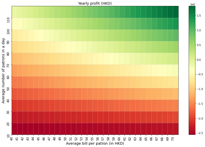
Quick Comment on the Plot
The plot visualizes the yearly profit of a café as a function of average foot traffic (number of patrons per day) and average bill size (spending per customer). Each cell represents the estimated profit based on the combination of these two factors, with color intensity indicating profit levels.
Key observations:
-
Low foot traffic (bottom rows) generally results in negative profits, regardless of the bill size, indicating that a minimum customer base is essential to cover fixed costs like rent and wages.
-
Higher foot traffic (top rows) leads to a positive profit zone, especially as the average bill size increases.
-
Profit Sensitivity: There is a clear transition from loss to profit as the average number of patrons and their spending increase, highlighting that both high traffic and a sufficient average bill are crucial for the café’s success.
This plot helps identify the break-even points, where running the café becomes profitable, and provides an intuitive visual guide for understanding how small changes in traffic or bill size affect overall profitability.
plt.figure(figsize=(12, 6))
foot_traffic = 90
df_mean_year_pnl.loc[foot_traffic].plot(marker='o', markersize=6, color='blue', lw=2, label='Profit')
plt.axhline(0, color='red', linestyle='--', lw=2, label='Break-even')
plt.grid(True, which='both', linestyle='--', linewidth=0.5, color='gray')
plt.xlabel("Average bill per patron (in HKD)", size=14)
plt.ylabel("Yearly profit (HKD)", size=14)
plt.title(f"Yearly profit in HKD (assuming {foot_traffic} daily patrons)", size=14)
plt.xticks(fontsize=12)
plt.yticks(fontsize=12)
plt.legend(loc='upper left', fontsize=12)
plt.tight_layout()
plt.show()
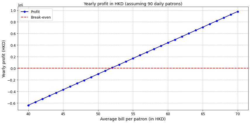
Brief Comment on the Plot
This plot illustrates the projected yearly profit of the café for a foot traffic level of 90 daily patrons, depending on the average spending per customer (bill size).
-
The red dashed line represents the break-even point, where profit is zero.
-
As we can see, with lower average bills, the café operates at a loss. However, once the average bill surpasses approximately HKD 52, the café crosses the break-even threshold and starts generating profit.
-
The plot shows the sensitivity of profitability to the bill size: even small increases in the average bill lead to significant improvements in yearly profit once the business crosses the break-even point.
This graph provides valuable insights into how bill size impacts the café’s financial performance, showing that profitability is highly dependent on maintaining a sufficiently high average spend per customer.
plt.figure(figsize=(12, 6))
avg_bill_patron_1 = 55
avg_bill_patron_2 = 65

# Plot the curves with different styles for better distinction
df_mean_year_pnl.T.loc[avg_bill_patron_1].plot(
    label=f"Average bill / patron: HKD {avg_bill_patron_1}", linestyle='-', marker='o', markersize=6, lw=2)
df_mean_year_pnl.T.loc[avg_bill_patron_2].plot(
    label=f"Average bill / patron: HKD {avg_bill_patron_2}", linestyle='--', marker='s', markersize=6, lw=2)

# Add the break-even line
plt.axhline(0, color='red', linestyle='--', lw=2, label='Break-even')

# Add gridlines and labels
plt.grid(True, which='both', linestyle='--', linewidth=0.5, color='gray')
plt.xlabel("Average number of patrons in a day", size=14)
plt.ylabel("Yearly profit (HKD)", size=14)
plt.title("Yearly profit in HKD (depending on number of daily patrons)", size=14)

# Customize ticks and legend
plt.xticks(fontsize=12)
plt.yticks(fontsize=12)
plt.legend(loc='upper left', fontsize=12)
plt.tight_layout()
plt.show()
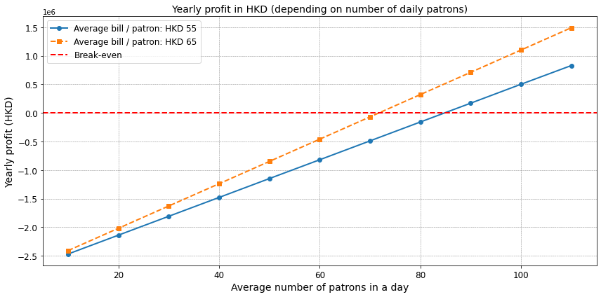
Brief Comment on the Plot
This plot visualizes the yearly profit of the café based on the number of daily patrons for two different average bill amounts: HKD 55 and HKD 65.
-
The solid line represents the yearly profit for an average bill of HKD 55, while the dashed line represents an average bill of HKD 65.
-
The red dashed line marks the break-even point, where the profit equals zero.
-
As expected, a higher average bill significantly boosts the profitability of the café, especially when the daily foot traffic increases.
-
For both bill amounts, the café operates at a loss at lower foot traffic levels, but as the number of daily patrons rises, profitability improves, with the break-even point being reached earlier for the HKD 65 bill compared to the HKD 55 bill.
Of course, pricing is competitive, and you may lose patrons by increasing price… which is not modeled at all here.
Overall, this simulation provides insights into the break-even points and profitability of a small café, highlighting how critical customer traffic and average spending are to the business’s financial health.
Simulation for 1 year of business, given a set of parameters
This final simulation runs multiple trajectories (1,000 simulations) of daily profit over the course of one year, given a specific set of parameters:
- Average foot traffic: 80 patrons per day
- Average bill per patron: HKD 59
- Daily rent: HKD 1,500
- Daily wages: HKD 1,200
Explanation of the Process
-
For each simulation, daily profit is computed based on observed daily foot traffic, which fluctuates around the set average (80 patrons), with variability of 20% (i.e., foot traffic is drawn from a normal distribution centered on 80 with a standard deviation of 16).
-
Daily profit is computed through the Bayesian Network, which conditions profit on variables such as foot traffic and daily sales, using the Joint Gaussian Distribution to account for dependencies between the variables.
-
The cumulative yearly profit is then calculated by summing up the daily profits for each simulation.
# simu of a given year for a given set of parameters:

FOOT_TRAFFIC = 80
model = build_model(
    average_bill=59,
    average_traffic=FOOT_TRAFFIC,
    daily_rent=1500,
    daily_wage=1200,
)

# Convert to Joint Gaussian Distribution (for inference)
jgd = model.to_joint_gaussian()


# Extract the mean and covariance matrix from the joint Gaussian distribution
mean = jgd[0]
covariance = jgd[1]
all_daily_pnl = []
NB_SIMU = 1000
for simu in tqdm(range(NB_SIMU)):
    daily_pnl = []
    dates = pd.date_range("2024-01-01", "2025-01-01")
    for date in dates:

        # Observed foot traffic
        observed_foot_traffic = np.random.normal(FOOT_TRAFFIC, 0.2 * FOOT_TRAFFIC)

        # Partition the joint distribution into blocks for conditioning
        mean_daily_sales = mean[3]      # Mean of DailySales
        mean_profit = mean[5]           # Mean of Profit

        # Extract variances and covariances needed for calculations
        cov_daily_sales = covariance[3, 3]  # Variance of DailySales
        cov_profit = covariance[5, 5]       # Variance of Profit

        # Extract covariances with observed variables
        cov_daily_sales_foot_traffic = covariance[0, 3]   # Covariance between DailySales and FootTraffic
        cov_profit_daily_sales = covariance[5, 3]         # Covariance between Profit and DailySales

        # Calculate conditional mean and variance for DailySales given the observed values
        conditional_mean_daily_sales = (
            mean_daily_sales +
            (cov_daily_sales_foot_traffic * (observed_foot_traffic - mean[0]) / covariance[0, 0])
        )

        # Calculate conditional variance for DailySales
        conditional_variance_daily_sales = (
            cov_daily_sales -
            (cov_daily_sales_foot_traffic ** 2 / covariance[0, 0])
        )

        # Now calculate the conditional mean and variance for Profit given the observed values of DailySales
        conditional_mean_profit_given_daily_sales = (
            mean_profit +
            cov_profit_daily_sales * (conditional_mean_daily_sales - mean_daily_sales) / cov_daily_sales
        )

        conditional_variance_profit_given_daily_sales = (
            cov_profit - (cov_profit_daily_sales ** 2) / cov_daily_sales
        )

        daily_pnl.append(conditional_mean_profit_given_daily_sales)

    all_daily_pnl.append(daily_pnl)
100%|█████████████████████████████████████| 1000/1000 [00:00<00:00, 1443.14it/s]
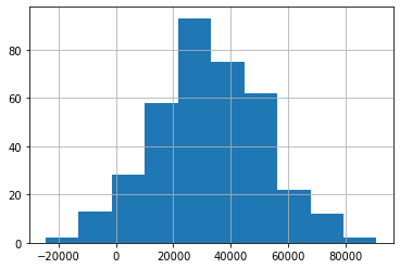
The histogram shows the distribution of cumulative yearly profits across all simulations. It helps assess the variability and risk of the business:
- The center of the distribution tells us the most likely range of outcomes.
- The spread (variance) reflects the financial uncertainty the café might face due to fluctuations in foot traffic and other factors.
pd.DataFrame(all_daily_pnl).cumsum().iloc[-1].hist()
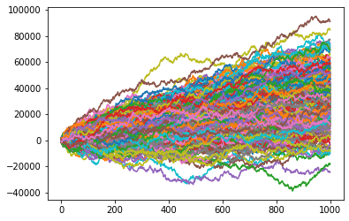
The trajectory plot shows the evolution of cumulative profit throughout the year for each simulation:
- It visualizes how profits evolve day-by-day, highlighting the range of possible trajectories.
- We observe significant variations, but overall patterns can emerge, such as the tendency to move into positive or negative profitability over time.
pd.DataFrame(all_daily_pnl).cumsum().plot(legend=False)
pd.DataFrame(all_daily_pnl).cumsum().iloc[-1].describe()
count      367.000000
mean     32584.652923
std      19024.309440
min     -24541.186664
25%      19872.687208
50%      32301.141206
75%      46470.777014
max      90926.336985
Name: 999, dtype: float64
Key Takeaways
- Profitability Uncertainty: The simulations indicate that while the café has potential to be profitable over the course of the year, variability in foot traffic creates uncertainty. The spread in both the histogram and trajectory plot shows the risk of losses in some scenarios, although the average outcome leans towards profitability.
- Break-even Point: Across the majority of simulations, the café does break even, but the risk of underperformance due to lower-than-expected foot traffic remains present.
Conclusion of the Study
In this simulation-based study of a café’s profit-and-loss model, we explored the business performance under daily fluctuations of key factors such as foot traffic and sales. The Bayesian network framework allowed us to capture and model the interdependencies between these variables, providing valuable insights into how the café is likely to perform over time.
Key insights include:
- The café’s profitability is highly sensitive to fluctuations in daily foot traffic, where even moderate changes can lead to significant profit variability.
- Incremental increases in the average bill per patron have a noticeable impact on the overall profitability, showcasing the importance of pricing.
- While the risk of financial underperformance remains, the model shows that under normal conditions, the café has a good chance of maintaining profitability.
Potential Follow-ups, Improvements, and Next Steps
-
Foot Traffic Seasonality: Incorporating seasonality into foot traffic would better capture real-world patterns, allowing us to simulate peak periods such as holidays or tourist seasons and to reflect the potential impact of these cycles on profits.
-
Uncertainty Reduction: To improve the accuracy of the simulations, gathering more data from real-world café operations would help refine key parameters like average bill size, customer flow, and fixed costs, reducing the model’s uncertainty.
-
Operational Costs Variability: Modeling fluctuations in operational costs, such as changes in raw material prices or labor costs, would provide a deeper understanding of how these factors impact profitability, especially during economic shifts.
-
Marketing Impact: Analyzing the potential effect of marketing initiatives on foot traffic and sales could provide insights into how different promotional efforts may enhance profitability.
In future work, incorporating these elements would enable a more holistic view of the café’s operations and give clearer forecasts of profitability under varied business conditions.